Chapter 13 Estimating forest parameters
Building on statistical concepts developed in Chapter 12, this chapter covers the basic steps and considerations needed to estimate forest parameters from a sample.118 In contrast to the finite population framework introduced earlier, this chapter adopts an infinite population perspective that better reflects how forest inventories are conducted in practice. Rather than sampling from a fixed list of discrete units, we place sample locations within the forest and summarize measurements made around each location. This shift shapes how sampling frames are defined, how units are selected, and how measurements are summarized.
The chapter closes with a section that embeds forest parameter estimation within a highly efficient tidyverse workflow, leveraging dplyr and tidyr functions covered in Chapters 8 and 9. We generalize and expand on these concepts and programming tools to accommodate more advanced forestry applications presented in subsequent chapters.
13.1 Sampling units for forestry applications
Collecting a sample used to estimate forest parameters is typically accomplished in three steps. First, sample locations, selected using some random mechanism, are placed within the forest. Second, a rule is used to select measurement trees around each location. Third, for each location, tree measurements are expanded to the desired per-unit-area basis and summarized to represent one observation within the sample. The most common rules for selecting measurement trees are plot sampling and point sampling.
Plot sampling is applied in many forestry applications, particularly in long-term monitoring efforts. A fixed-area plot is positioned at each sampling location, and trees within the plot boundary are measured. A sampling location can define the center for a circular plot, a corner for a rectangular plot, or the position for more complex plot shapes and configurations such as plot clusters or nested plots of different sizes. Under plot sampling, a tree’s selection probability is proportional to the area of the plot used for sampling.
Point sampling is also a common approach to tree selection and a popular method for cruising timber. Under point sampling, the probability of selecting a tree for measurement is conditional on some function of its size. For this reason, the approach is often called probability proportional to size (PPS) sampling. Depending on the survey objectives, compared with plot sampling, point sampling can offer greater efficiency from both a field-effort and statistical standpoint. In general, there are gains in efficiency when trees are preferentially selected for measurement based on a size attribute related to the parameter of interest. For example, if we’re interested in estimating volume, it’s more efficient to select measurement trees proportional to their basal area (because basal area and volume are strongly related). However, if we’re interested in estimating tree density (i.e., number of trees per unit area) or growth rates, plot sampling would be the preferred approach.
The next section connects forestry applications with concepts from Chapter 12. Specifically, we introduce the areal sampling frame, which takes the place of the list sampling frame introduced in Section 12.2.2. For the applications covered here, the areal sampling frame is used for both plot and point sampling. Then, because it’s conceptually easier, we introduce plot sampling, expansion factors, boundary effects, and other related topics. This is followed by point sampling and how expansion factors and other sampling considerations change under this tree selection rule.
13.2 Areal sampling frame
Recall from Section 12.2.2 that SRS and related probability sampling methods require a sampling frame from which the sample is selected. In the examples presented in the previous chapter, the sampling frame is a list of all population units from which sample units are randomly selected. For instance, in the Harvard Forest biomass analysis described in Section 12.3.5, the frame was constructed by overlaying a grid of equal-sized squares across the forest extent (Figure 12.3). This grid delineated the \(N\) population units, with indices \(1\) through \(N\), and sampling units were selected by drawing \(n\) random integers in that range. This is a valid and intuitive approach to sample selection.
Geographic information systems (GIS) and R’s spatial data packages (see, e.g., Pebesma and Bivand (2023); Brunsdon and Comber (2019)) can be used to tessellate—or grid—the geographic extent of a population using equal-area, non-overlapping shapes such as rectangles, as in the Harvard Forest example. Creating such grids is straightforward at a computer. However, logistical challenges, such as locating sampling unit boundaries and measuring trees within selected units in the field, often make these approaches impractical in forestry applications.
A more common approach in forestry is to use an areal sampling frame. This frame allows selection of any point location defined by geographic coordinates (e.g., longitude and latitude) within the population extent, usually outlined by one or more boundary polygons. Sampling locations are points placed using a random mechanism within this area. Each observation is a per-unit-area summary of the variable at that location, computed from all trees selected by the sampling rule, and treated as the value at that location.
Selecting discrete sampling units from a finite list sampling frame differs from selecting points from the infinitely many locations within an area. Fortunately, much of the statistical theory needed for valid inference is shared between list and areal frames. However, using an areal frame brings additional survey design, data collection, and analysis considerations, which are covered in this and subsequent chapters.
Using an areal frame for SRS introduces both statistical and logistical challenges. When sampling locations are randomly distributed, plots may overlap spatially—particularly with fixed-area plots if locations fall too close together. The same trees can then be measured more than once, increasing redundancy and reducing statistical efficiency. This doesn’t violate SRS assumptions or the validity of design-based estimators, but it can yield less informative samples. Logistically, it can also be inefficient to navigate to a random set of widely dispersed locations in the field, especially in forested or rugged terrain. To address these issues, forest inventories typically use systematic designs in which sampling locations are spaced evenly across the population extent. To preserve key probability sampling properties, the systematic grid is positioned using a random mechanism. See Figure 2.2 for illustration and Chapter 15 on systematic sampling for further details.
Despite these practical considerations, we continue to use SRS in this chapter for both plot and point sampling because the concepts introduced—defining sampling units, expanding tree-level measurements, and summarizing observations—are foundational and largely design-agnostic. Moreover, several of the more complex designs introduced in subsequent chapters adopt or extend estimators originally developed under SRS. The ideas we establish here provide the grounding needed to understand and implement the more advanced forest sampling strategies that follow.
13.2.1 Finite population correction
While we emphasized the role of the finite population correction in Section 12.3, it’s rarely applied in forest inventory. The FPC is relevant when sampling is conducted from a list sampling frame, where the population is finite, its size (i.e., \(N\)) is known, and each unit is discrete and identifiable. In this case, the correction reduces the standard error because, once selected, a unit is no longer eligible for reselection.
In contrast, with an areal sampling frame the number of possible sampling locations is effectively infinite, and there is no predefined finite set of discrete units. A sampling location can occur anywhere within the geographic extent. Because of this, the conditions required for applying the FPC don’t hold, and the correction is not used when estimating standard errors for samples selected from an areal frame.
13.3 Plot sampling
As noted at the beginning of this chapter, plot sampling is a common approach for collecting forest inventory data used to estimate population parameters. Fixed-area plots, often circular or rectangular, are established at sampling locations selected from an areal sampling frame. All trees within the plot boundary that belong to the population of interest are then measured. The criteria for determining whether a tree is “in” the plot are typically defined in the field protocol—for example, a standing tree is measured if the center of its stem at DBH falls within the plot boundary.
The survey objectives define the population(s) of interest. For example, in a timber cruise, we might measure only marketable trees—live stems of a certain DBH, species, and log quality. In an Emerald Ash Borer (EAB) forest health assessment, we might measure live and dead ash species. In a regeneration survey, we might measure seedlings and saplings of desirable species.
In practice, we’re almost always interested in estimating parameters for multiple populations. These populations often differ in ways that guide how they’re sampled. For example, tree density (number of trees per unit area) can vary greatly among populations. Suppose we’re assessing both regeneration potential and timber volume in a naturally regenerated, uneven-aged stand. These two stand components—regeneration and overstory—can be viewed as distinct populations. Such stands typically contain far more seedlings and saplings than large overstory trees on a per-area basis. Thus, an ideal large plot size for overstory trees would likely result in excessive time spent measuring small regeneration stems, while a small plot suited for regeneration would include too few overstory trees to reliably estimate timber volume with a feasible number of plots.
The solution is to co-locate plots sized appropriately for each population of interest, often by nesting smaller plots within larger ones. This might look like one or more 1/1000-th acre regeneration plots nested within a 1/20-th acre overstory plot. Smaller nested plots are often referred to as subplots.
When using plot sampling, each tree’s selection probability is proportional to the area of the plot in which it’s measured. More specifically, this probability equals the plot area divided by the geographic extent of the population. These ideas are further developed in Section 13.3.1 and illustrated in Section 13.3.6. They’re key to expanding tree measurements to a per-unit-area basis (e.g., per acre or per hectare) and computing plot-level summaries that represent one observation within the sample.
13.3.1 Expansion factors and plot-level summaries
In most forestry applications, estimates are expressed on a standard per-unit-area basis (i.e., acre or hectare). This means that at some point in the analysis we need to scale tree measurements to the desired per-unit-area basis. For example, recall from Section 12.1.5 that we were interested in estimating the average biomass (Mg/ha) in the Harvard Forest. However, because our sampling units (i.e., plots) were 0.25 ha, we first multiplied the total tree biomass measured on each 0.25-ha unit by 4 (i.e., 1/0.25) to express it on a per-hectare basis. Here, the value 4 is referred to as an expansion factor. An expansion factor is a value used to scale measurements from one area basis to another. In the Harvard Forest analysis, the individual tree measurements were summarized to the 0.25-ha plot in advance, and the expansion factor was then applied to the plot-level summaries to arrive at the desired per-hectare expression.

FIGURE 13.1: Two perspectives of measurement tree selection using a fixed-area circular plot. (a) Plot-centered, where the circle identifies the plot boundary. (b) Tree-centered, where circles identify each tree’s inclusion zone with solid and dashed lines corresponding to measurement and non-measurement trees, respectively.
To better understand expansion factors, it’s helpful to consider two perspectives for measurement tree selection. In the preceding section, our description of measurement tree selection takes a plot-centered perspective—that is, as illustrated in Figure 13.1(a), a plot boundary is established at a sampling location and trees inside the plot are measured. Alternatively, we can take a tree-centered perspective, in which an imaginary plot identical in shape and size to the one intended for the sampling location is established using each tree’s location. The tree’s imaginary plot is called its inclusion zone and is illustrated in Figure 13.1(b).119 All trees with inclusion zones containing the sampling location are measured. Notice in Figure 13.1 that both perspectives result in the same set of measurement trees.
The \(j\)-th tree’s measurements are scaled to a per-unit-area basis using the tree expansion factor, or tree factor (TF) for short, defined as \[\begin{equation} \text{TF}_j = \frac{\text{unit area}}{\text{inclusion zone area}_j}. \tag{13.1} \end{equation}\]
In most applications, the unit-area numerator is 43,560 (ft\(^2\)/ac) or 10,000 (m\(^2\)/ha), and the denominator is the \(j\)-th tree’s inclusion zone area in ft\(^2\) or m\(^2\). Regardless of the measurement system or chosen base units, TF is the number of trees per unit area that the given measurement tree represents.
As illustrated in Figure 13.1, under plot sampling a tree’s inclusion zone equals the plot area used to sample the population to which the tree belongs. Hence, following (13.1), all trees measured on a given plot size will have the same TF.
We’re careful to note “population” because it’s often the case that different populations are measured using different plot sizes within the same survey effort. For example, following the description of overstory and regeneration plots in Section 13.3, a tree measured on the 1/20-th-acre (0.05 ac or 2,178 ft\(^2\)) fixed-area overstory plot will have a 0.05-acre inclusion zone and represent \(\text{TF}\) = 43,560/2,178 = 20 trees per acre. Similarly, a seedling or sapling measured on the 1/1,000-th-acre (0.001 ac or 43.56 ft\(^2\))120 subplot will have a 0.001-acre inclusion zone and represent \(\text{TF}\) = 43,560/43.56 = 1,000 trees per acre.
A per-unit-area expansion for the \(j\)-th tree’s continuous or binary measurement (e.g., basal area, volume, biomass, logs, live/dead) is \[\begin{equation} y_j \left(\text{units}/\text{unit area}\right) = y_j \left(\text{units}/\text{tree}\right)\cdot \text{TF}_j \left(\text{trees}/\text{unit area}\right), \tag{13.2} \end{equation}\] where \(y_j\) represents the tree-level measurement in the given units.
For example, following (13.2), suppose the \(j\)-th tree measured on a 0.05-acre plot had a DBH of 10 inches. Given \(\text{TF}_j=20\) trees per acre, its basal area per acre is \[\begin{align*} \text{BA}_j \left(\text{ft}^2/\text{acre}\right) &= \left(c\cdot \text{DBH}_j^2\right)\left(\text{ft}^2/\text{tree}\right)\cdot \text{TF}_j \left(\text{trees}/\text{acre}\right)\\ &= 0.005454 \cdot 10^2 \cdot 20 \\ &= 10.908, \end{align*}\] where \(c = 0.005454 = \pi/(144\cdot 4)\).121122
Next, suppose that same tree had a volume \(v_j\) of 10.4 ft\(^3\); then, again following (13.2), its expanded volume is \[\begin{align*} v_j \left(\text{ft}^3/\text{acre}\right) &= v_j \left(\text{ft}^3/\text{tree}\right)\cdot \text{TF}_j \left(\text{trees}/\text{acre}\right)\\ &= 10.4 \cdot 20 \\ &= 208. \end{align*}\]
The individual tree measurements, expanded to a per-unit-area basis, are then combined to form a plot-level summary. For the \(i\)-th sampling location, the general expression for a per-unit-area plot-level summary is \[\begin{equation} y_i = \sum_{j=1}^{m_i} y_{ij} \cdot \text{TF}_{ij}, \tag{13.3} \end{equation}\] where \(y_{ij}\) represents the \(j\)-th tree’s measurement in the chosen units, \(\text{TF}_{ij}\) is its tree factor, and \(m_i\) is the number of measurement trees on plot \(i\).123
Applying this general formula to specific variables, the plot-level summary for number of trees per unit area is \[\begin{equation} \text{Trees}_i = \sum_{j=1}^{m_i}\text{TF}_{ij}, \tag{13.4} \end{equation}\] where the per-tree quantity \(y_{ij}\) in (13.3) is implicitly 1 for a counted tree. For plot sampling, this summation reduces to \(m_i\!\cdot\!\text{TF}\), where TF is the constant tree expansion factor for all trees measured on the plot.124
Similarly, the \(i\)-th sampling location’s per-unit-area summaries for other variables are obtained by summing the per-unit-area contributions of its measured trees. For example, following (13.3), the plot-level summaries for basal area and volume per unit area are \[\begin{equation} \text{BA}_i = \sum_{j=1}^{m_i} c\cdot \text{DBH}_{ij}^2 \cdot \text{TF}_{ij}, \tag{13.5} \end{equation}\] and \[\begin{equation} v_i = \sum_{j=1}^{m_i} v_{ij}\cdot \text{TF}_{ij}. \tag{13.6} \end{equation}\]
In this notation, \(\text{Trees}_i\), \(\text{BA}_i\), and \(v_i\) are simply instances of \(y_i\) from Section 12.3, with \(i\) indexing sample observations. These per-plot summaries serve as the observations for subsequent sample-based estimation.
13.3.2 Sample-based estimates
For \(n\) sampling locations, the corresponding \(n\) per-unit-area plot-level summaries of a given variable (see Section 13.3.1) serve as the sample observations used to estimate population parameters via the estimators described in Section 12.3. Following the notation introduced in Section 12.3, the \(n\) plot-level summaries are denoted \(y_i\), for \(i=1,2,\ldots,n\), and are used to compute the sample mean, standard error of the mean, and confidence intervals using (12.15), (12.21), and (12.31), respectively.
These plot-level summaries—one per sampling location—form the essential link between tree-level measurements and population-level inference.
Continuing the example from Section 13.3.1, per-acre sample-mean estimates for tree density, basal area, and volume are \[\begin{equation} \overline{\text{Trees}} = \frac{\sum_{i=1}^{n}\text{Trees}_i}{n}, \tag{13.7} \end{equation}\] \[\begin{equation} \overline{\text{BA}} = \frac{\sum_{i=1}^{n}\text{BA}_i}{n}, \tag{13.8} \end{equation}\] and \[\begin{equation} \bar{v} = \frac{\sum_{i=1}^{n}v_i}{n}. \tag{13.9} \end{equation}\] These are simply variable-specific instances of \(\bar{y}\), and their standard errors and confidence intervals follow directly from (12.21) and (12.31).
Estimates for population totals (e.g., total number of trees, basal area, or volume) are obtained by scaling each per-unit-area mean by the total forest area. This matches the approach in Section 12.3.3, where the population size \(N\) is replaced by the forest area \(A\), expressed in the same units as the per-unit-area estimates. Computation of means and totals for several parameters are illustrated in Section 13.3.6.
The tree-centered perspective developed above continues to offer practical benefits. First, as shown in Section 13.3.1, it aids in introducing tree expansion factors. Second, from a practical computing standpoint, it supports a single analytical workflow (Section 13.6) that yields population parameter estimates for both plot and point sampling data. Third, it clarifies how forest sampling based on an areal sampling frame connects with broader survey sampling theory (see, e.g., Grosenbaugh (1958), Oderwald (1981), Roesch et al. (1993), and Gregoire and Valentine (2008)). Fourth, as explored in subsequent sections, it helps us recognize and address statistical issues that can arise during implementation.
13.3.3 Boundary effects
The validity of plot and point sampling requires that the probability of selecting a tree for measurement is proportional to the tree’s inclusion zone. If any portion of a tree’s inclusion zone falls outside the forest boundary, then that tree has a lower than expected probability of selection. This reduced probability can result in biased estimates, referred to as boundary slopover bias. This bias can, and should, be corrected in the field using methods found in most forest measurement books (see, e.g., Burkhart et al. (2018), Kershaw et al. (2016), and Gregoire and Valentine (2008) for an in-depth tour of methods proposed to correct boundary slopover bias).
Below, we review the mirage and walkthrough methods. Both are easy to implement and common in practice. They effectively correct for those trees with inclusion zones that extend beyond the boundary. We introduce the methods using circular plots, but they can also be applied for non-circular plots.
The mirage method was proposed by Schmid (1969).125 The method can be applied when the boundary near the plot in question is straight (or made up of straight segments with well-defined corners) and you are able to work outside the boundary. The method is implemented using the following steps.
- Establish the plot center. Measure all trees that fall inside the plot and are also inside the boundary. If any portion of the plot is over the boundary, then implement Step 2.
- Determine the bearing with the shortest distance \(d\) from the plot center to the boundary. Establish a “mirage” (i.e., temporary) plot center along the bearing at distance \(d\) outside the boundary. From that mirage plot center, measure all trees that fall inside the mirage plot and also inside the boundary. Add these mirage plot measurement trees to the measurement trees recorded in Step 1.
Figure 13.2 shows three fixed-area circular plots with increasing amounts of boundary overlap. Following Step 2 above, the mirage sampling locations are established at a distance \(d\) outside the boundary. The shaded regions within each sampling location plot show how many times each measurement tree should be recorded. Notice that trees falling within the overlap between the sampling location plot and the mirage plot are recorded twice.

FIGURE 13.2: Three fixed-area circular plots with increasing boundary overlap. Boundary indicated by the dashed line. Mirage plots outlined with dotted line.
Consider Figure 13.3 to build some intuition for how the mirage method works. Like Figure 13.1, it shows measurement tree selection from both a plot- and tree-centered perspective. Figure 13.3(a) shows a plot with boundary overlap and two measurement trees. Following the mirage method, Tree 1 is recorded twice because it falls within the region where the mirage plot overlaps the sampling location plot. Tree 2 is recorded only once because it doesn’t fall within the overlap. Double counting Tree 1 effectively corrects for the fact that its inclusion zone is reduced by the portion extending beyond the boundary.
Given this notion, consider the corresponding tree-centered view in Figure 13.3(b), where a mirage tree inclusion zone has been established for each measurement tree. For a given tree, notice the inclusion zone area outside the boundary is equal to the mirage inclusion zone area inside the boundary—effectively correcting the inclusion zone area reduction, or making it whole.
It might help to think of the portion of a tree’s inclusion zone area that extends beyond the boundary as being folded back onto itself along the boundary. The sampling location falls within Tree 1’s inclusion zone and inclusion zone correction region; hence, that tree is recorded twice. For Tree 2, the sampling location falls within its inclusion zone but not its inclusion zone correction region; hence, it’s recorded only once.

FIGURE 13.3: Plot-centered and tree-centered view of the mirage method using two example trees.
The walkthrough method was developed by Ducey et al. (2004). This method follows the same basic principles as the mirage method but is more general and works well even if the boundary near the plot in question is not straight, or if you are not able to work outside the boundary. The method is implemented using the following steps.
- Establish the plot center. Measure all trees that fall inside the plot and are also inside the boundary.
- Identify each tree in the plot that is closer to the boundary than to the plot center. For each of these trees, take the bearing from the plot center to the tree and also measure the distance \(d\) from the plot center to the tree. Then, following this bearing, walk from the tree for distance \(d\). The point at distance \(d\) from the tree (i.e., where you stop walking) is called the “walkthrough point.” If the walkthrough point is outside the boundary, then the tree is recorded twice; otherwise, the tree is recorded only once. It doesn’t matter how many times you cross the boundary on the way to the walkthrough point—it’s whether the walkthrough point is inside or outside the boundary that determines if the tree is recorded once or twice. It’s only necessary to walk to the walkthrough point if it’s not obvious whether the point is inside the boundary.
Consider the example in Figure 13.4. Here, a fixed-area circular plot center falls near a boundary. Six trees fall within the plot and boundary. Each tree’s walkthrough point is also identified in the figure. In practice, only Trees 1, 2, 5, and 6 would likely be considered using the walkthrough method, since Trees 3 and 4 are clearly closer to the plot center than to the boundary. Trees 1 and 6 have walkthrough points outside the boundary, so they’re recorded twice. The other trees have walkthrough points within the boundary and are recorded only once.

FIGURE 13.4: Fixed-area circular plot indicated by the solid line that overlaps a boundary indicated by the dashed line. Six trees fall in the plot. Arrows indicate direction and distance to walkthrough points denoted with asterisked tree number.
13.3.4 Slope corrections
Forest parameters are reported on a horizontal land area basis (e.g., tons per hectare or volume per acre). Horizontal areas are delineated on the horizontal plane. The land surface, with all its interesting terrain features, can be projected onto the horizontal plane; however, this projection results in some distortion that we must consider. The key issue here is that a fixed-area plot established on a slope (i.e., oblique plane) has a smaller area when projected onto the horizontal plane. Hence, tree factors computed for horizontal plot areas should not be applied to trees measured on sloped plots. Plots that fall on a slope require slope correction prior to use in estimation.
Let’s build some intuition about the need for slope correction. Say we’re using a fixed-area circular plot with radius \(R\) to conduct our cruise. If this circular plot is established on an oblique plane with slope \(\alpha\), the plot shape when projected onto the horizontal plane becomes an ellipse with major radius \(R\), minor radius \(R^\ast = \cos(\alpha)R\), and area \(\pi RR^\ast\) (which is smaller than \(\pi R^2\)). This relationship is illustrated in Figure 13.5(a), where the upper sloped plot area is a circle with radius \(R\) that becomes an ellipse when projected down onto the horizontal plane. Importantly, the area of this projected ellipse is smaller than \(\pi R^2\)—hence, applying the tree factor computed assuming an area of \(\pi R^2\) will cause downward bias in resulting estimates.
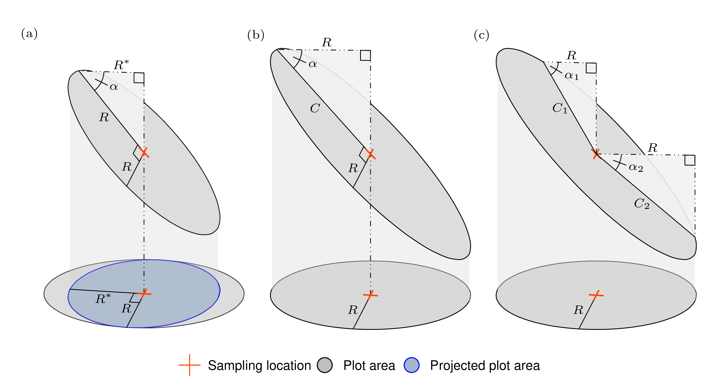
FIGURE 13.5: Illustration of how fixed-area plot dimensions change when projected between the horizontal (lower) and oblique (upper) planes. (a) Plot area when projecting a circular plot on an oblique plane onto the horizontal plane. (b,c) Examples used to find the oblique plane plot’s radius and critical distance given \(R\) and slope angle \(\alpha\).
There are a few approaches for slope correction. The most general is to ensure that all measurements are made using horizontal distance, not the distance along the oblique plane. For example, if you had a circular plot that falls on an oblique plane with slope \(\alpha\), the plot shape becomes an ellipse with minor axis radius \(R\) perpendicular to the slope, major axis radius \(C = R/\cos(\alpha)\) parallel with the slope, and area \(\pi R C\). Once projected to the horizontal plane, this elliptical plot has the desired plot area of \(\pi R^2\) (i.e., \(C = R\) when \(\alpha = 0\)). This projection and associated dimensions are illustrated in Figure 13.5(b).
In practice, we don’t actually lay out an elliptical slope plot—that would be painful. Rather, we check if each tree around the sloped plot center is within the corresponding horizontal plot radius. If a tree is within the horizontal plot radius, then it’s a measurement tree.
Checking if a tree is “in” or “out” of the elliptical plot is straightforward once you recognize that it amounts to computing a right triangle’s hypotenuse length with known angle \(\alpha\) and adjacent side \(R\), then comparing the hypotenuse length to the distance from the plot center to the tree in question. We’ll call this hypotenuse \(C\), the tree’s critical distance. If the slope distance from the plot center to the tree is smaller than the tree’s critical distance, then it’s a measurement tree.
A tree’s critical distance is determined by the slope between the plot center and the tree’s location. The \(j\)-th tree has critical distance \(C_j = R/\cos(\alpha_j)\), where \(\alpha_j\) is the slope from the plot center to the center of the tree’s stem (slope measured parallel to the ground at the tree’s stem center). This slope can be found using a clinometer or laser rangefinder that is able to calculate slope.
For example, consider Figure 13.5(c), and say we’d like to compute a critical distance for a tree positioned along the direction indicated by line \(C_1\). Using a clinometer, you find the slope \(\alpha_1\) is 30 degrees. The cruise protocol calls for a circular plot with \(R = 26.33\) (ft) (the horizontal distance radius of a 1/20-th acre plot). The tree’s critical distance is then \(C_1 = R/\cos(\alpha_1) = 26.33/\cos(30) = 30.4\) (ft).126 So, the tree must be within \(30.4\) (ft) of the plot center (measured along the slope) to be a measurement tree.
Now say the next tree is positioned along the \(C_2\) line. Using a clinometer, you find the slope \(\alpha_2\) is 40 degrees. The tree’s critical distance is \(C_2 = R/\cos(\alpha_2) = 26.33/\cos(40) = 34.37\) (ft).
The slope correction approach described above is general and works even when the slope is not constant across the plot area. Many modern laser rangefinders report horizontal distance and hence automatically correct for slope. Using such a device, simply measure the horizontal distance from the plot center to each possible measurement tree. Those trees with horizontal distance (to the tree center) less than \(R\) are measurement trees. These results will match the time- and math-intensive approach of finding each tree’s critical distance. This approach is also the most commonly used in national forest inventories and similar inventories where accuracy and repeatability are key.
There are two other approaches to slope correction often seen in practice.
Radius adjustment uses a larger circular plot on the slope that, when projected onto the horizontal plane, has area \(\pi R^2\) (Bryan 1956).
Tree factor adjustment uses a circular plot with radius \(R\) on the slope but computes a plot-specific tree factor that accounts for the resulting smaller plot area when projected onto the horizontal plane (Beers 1969).
Both approaches require a measurement that captures the overall plot slope.
To apply the radius adjustment approach, establish a circular plot on the slope with radius \(R^\ast = R/\sqrt{cos(\alpha)}\). This circular plot defined by radius \(R^\ast\) on the slope will be an ellipse with area \(\pi R^2\) when projected onto the horizontal plane. This works because the inclusion zone area of the projected ellipse equals that of the intended plot on the horizontal plane. This approach might be a good option for a timber cruise as it allows you to keep a constant radius, which greatly simplifies identifying measurement trees using a tape from the plot center. Foresters using this approach often rely on a table that provides a scaling factor for \(R\) given different slope ranges.
For example, if your cruise protocol calls for a circular plot with \(R=26.33\) (ft) (horizontal distance) and the plot falls on a \(\alpha = 30\) (degree) slope, the adjusted radius is \(R^\ast = R/\sqrt{\cos(\alpha)} = 28.3\) (ft) or using the equivalent scaling factor \(R^\ast = r^\ast R\) where \(r^\ast = 1/\sqrt{cos(\alpha)} = 1.07\). To create your own scaling factor table to take into the field, compute \(r^\ast\) for a range of slopes (see Exercise 13.12).
To apply the tree factor adjustment approach, establish a circular plot on the slope with radius \(R\) as if it were on the horizontal plane. Because the area of this slope plot is smaller than \(\pi R^2\) when projected onto the horizontal plane, the tree factor for measurement trees needs to increase accordingly. Specifically, the tree factor for measurement trees on the slope plot is \(\text{TF}^\ast = \text{TF}/\cos(\alpha)\), where \(\text{TF} = \text{unit area}/(\pi R^2)\) (following (13.1)) or equivalently \(\text{TF}^\ast= \text{unit area}/(\pi \cos(\alpha) R^2)\), where the denominator is the area of the horizontally projected ellipse, i.e., the blue area in Figure 13.5(a).
This approach is also easy to implement, but it requires that you record all plot slopes so you can compute corresponding tree factors after the cruise. As an example, say your horizontal plot radius is \(R=26.33\) (ft), which results in a \(\text{TF} = 43560 / (\pi 26.33^2) = 20\). The tree factor for trees measured on the oblique plot with a slope of 30 (degrees) and \(R=26.33\) (ft) is \(\text{TF}^\ast = \text{TF}/\cos(\alpha) = 23.09401\).
13.3.5 Effect of plot size on variance
Plot size, i.e., the area covered by the sampling unit, affects variance and, in turn, inferences that involve variance such as confidence intervals and sample size calculations. For many variables measured in forestry applications, the variance of measurements collected on small plots is greater than the variance of measurements collected on larger plots. For example, the variance in biomass measurements (Mg/ha) taken on 0.25 ha plots will be larger than the variance in biomass measurements (Mg/ha) on 0.5 ha plots.
Large plots tend to have smaller variance because they average over small-scale horizontal forest structure caused by factors such as competition, harvesting, windthrow, disease, or fire. The effect of plot size on variance diminishes as stand structure becomes more uniform. For example, we expect a plantation to have a weaker plot size to variance relationship compared with structurally complex mixed-species uneven-aged stands.
Freese (1962) offers the following equation to approximate the relationship between plot size and variance. \[\begin{equation} s_2^2 = s_1^2 \sqrt{\frac{a_1}{a_2}}, \tag{13.10} \end{equation}\] where plot size \(a_1\) has variance \(s^2_1\) and plot size \(a_2\) has variance \(s^2_2\). One can replace the variances in (13.10) with their corresponding coefficients of variation (i.e., \(CV_1 = s^2_1/\bar{y}_1\) and \(CV_2 = s^2_2/\bar{y}_2\)).
For example, following (13.10), if the variance of pulpwood volume per acre on 1/4-acre plots is \(s_1^2 = 50\), the variance in pulpwood volume per acre on a 1/10-acre plot is approximately \[\begin{align*} s_2^2 &= 50\sqrt{\frac{0.25}{0.1}}\\ & = 79.06. \end{align*}\]
Although plot size is often chosen based on experience or an existing field sampling protocol, the relationship between plot size and expected variance can provide an approach to select plot size and sample size based on allowable error and cost constraints. Cost comes into play here because “time is money”—to reach the same standard error, there are trade-offs between sampling more small plots versus fewer large plots.
For example, if travel time between many small plots is large relative to the time needed to take measurements on fewer large plots, one would favor a sampling design where fewer large plots are selected.
13.3.6 Illustration
Figure 13.6 shows a toy dataset that we’ll use to illustrate estimation via plot sampling. The figure shows a forest area (1.32 ac) that delineates tree populations of interest. The forest is divided into two stands (Stand 1 is 0.64 ac and Stand 2 is 0.68 ac), and within each a distinction is made between overstory and regeneration trees. This partitioning allows us to define at most four populations: Stand 1 overstory trees, Stand 1 regeneration trees, Stand 2 overstory trees, and Stand 2 regeneration trees.
These are simulated data, meaning we created them, and as a result we have measurements on all trees, i.e., a census. These measurements allow us to compute the population parameter values of interest that are given in Table 13.1. For instructional purposes, we can compare these parameter values to their corresponding estimates—something we can’t do when sampling a real population.127

FIGURE 13.6: Toy dataset used to illustrate sample-based estimation.
| Stand | Trees/ac | Basal area (ft\(^2\)/ac) | Volume (ft\(^3\)/ac) | Trees/ac |
|---|---|---|---|---|
| 1 | 78.210 | 64.506 | 1809.93 | 782.10 |
| 2 | 73.206 | 27.907 | 643.04 | 732.06 |
The sample comprises trees measured on six overstory plots with accompanying regeneration subplots. Overstory and regeneration plots are circular fixed-areas with 24 ft and 6.8 ft radii, respectively. Plot sampling locations were selected at random (i.e., SRS) from each stand’s areal sampling frame and serve as the overstory plot centers. Regeneration subplots were located 12 ft east of overstory plot centers.128
On overstory plots, species, DBH (in), and height (ft) for all trees with DBH \(\ge\) 2 in were measured. Additionally, volume (ft\(^3\)) was estimated for measurement trees using allometric equations provided in Honer (1967). On regeneration subplots, the number of trees by species with height greater than 2 ft and DBH \(<\) 2 in were recorded.

FIGURE 13.7: A sample from the populations shown in Figure 13.6. The sample comprises three fixed-area circular overstory plots randomly located within each stand. Regeneration subplots are nested within overstory plots.
This illustration steps through the calculations used to estimate number of trees, basal area, and volume per acre, as well as their stand totals. To keep the focus on these steps, we’ll initially limit our analysis to the overstory plot data in Stand 1. Later in Section 13.6, we develop an efficient workflow for both stands and apply it to estimate parameters for both the overstory and regeneration layers.
Table 13.2 provides overstory tree measurements for the three Stand 1 plots. Notice in Figure 13.7, there are no overstory trees on Plot 2 in Stand 1. It’s critical that the absence of trees at a sampling location be included in subsequent estimates—meaning a plot with no trees is part of the sample, reflects a characteristic of the population, and needs to be included as a zero when computing population parameter estimates.
We include a line for Plot 2 in Table 13.2 with zero DBH and volume values to remind us to include these values in subsequent computations.
| Plot | DBH (in) | Volume (ft\(^3\)) |
|---|---|---|
| 1 | 11.3 | 17.8 |
| 1 | 9.8 | 14.5 |
| 1 | 10.7 | 17.9 |
| 2 | 0.0 | 0.0 |
| 3 | 14.8 | 33.6 |
| 3 | 15.4 | 36.6 |
| 3 | 13.1 | 28.9 |
We divide the estimation process into two steps, which were covered in Sections 13.3.1 and 13.3.2, respectively.129 First, compute plot-level summaries for each variable following (13.3). The plot-level summaries comprise each plot’s expanded and summarized tree measurements expressed on a per-unit-area basis (these are the sample observations). Second, use the plot-level summaries to compute the desired population parameter estimates (see Section 13.3.2).
Computing the plot-level summaries begins with calculating the TF used by all overstory trees measured on the 24 ft radius circular fixed-area plot. Following (13.1), the TF is \[\begin{align*} \text{TF} \left(\text{trees}/\text{ac}\right) &= \frac{\text{unit area} \left(\text{ft}^2/\text{ac}\right)}{\text{inclusion zone area} \left(\text{ft}^2/\text{tree}\right)}\\[0.5ex] &= \frac{43560}{\pi\cdot R^2} = \frac{43560}{\pi\cdot 24^2}\\ &= 24.07219, \end{align*}\] where \(R\) is the plot radius. This tree factor tells us that each tree measured on an overstory plot represents 24.07 trees per acre.
Next, we compute trees per acre for each of the \(n\) = 3 plots. Referring to Table 13.2 to get the number of trees on each plot and following (13.4), the plot-level trees per acre are \[\begin{align*} \text{Plot 1:}&\; \sum^3_{j=1}\text{TF}_j = 3\cdot \text{TF} = 72.21656 \left(\text{trees}/\text{ac}\right),\\ \text{Plot 2:}&\; \text{TF}\cdot 0 = 0\left(\text{trees}/\text{ac}\right),\\ \text{Plot 3:}&\; \sum^3_{j=1}\text{TF}_j = 3\cdot \text{TF} = 72.21656 \left(\text{trees}/\text{ac}\right), \end{align*}\] where \(j\) is the tree index. Notice in the calculations above, because the TF is a constant we pull it out of the summation and drop its subscript.
Using DBH measurements in Table 13.2 and following (13.5), the plot-level basal area per acre is \[\begin{align*} \text{Plot 1:}&\; \sum^3_{j=1}c\!\cdot\!\text{DBH}^2_j\!\cdot\!\text{TF}_j = c\cdot (11.3^2\!+\!9.8^2\!+\!10.7^2)\!\cdot\!\text{TF}\\[-0.5em] &\qquad\qquad\qquad\quad\,\, = 44.4048 \left(\text{ft}^2/\text{ac}\right),\\ \text{Plot 2:}&\; \text{TF}\!\cdot\!0 = 0 \left(\text{ft}^2/\text{ac}\right),\\ \text{Plot 3:}&\; \sum^3_{j=1}c\!\cdot\!\text{DBH}^2_j\!\cdot\!\text{TF}_j = c\cdot\!(14.8^2\!+\!15.4^2\!+\!13.1^2)\!\cdot\!\text{TF}\\[-0.5em] &\qquad\qquad\qquad\quad\,\, = 82.42499 \left(\text{ft}^2/\text{ac}\right), \end{align*}\] where \(c = 0.005454\).130 Using volume measurements in Table 13.2 and following (13.6), the plot-level volume per acre is \[\begin{align*} \text{Plot 1:}&\; \sum^3_{j=1}v_j\!\cdot\!\text{TF}_j = (17.8\!+\!14.5\!+\!17.9)\!\cdot\!\text{TF}\\[-0.5em] &\qquad\qquad\;\,\,\, = 1208.42369 \left(\text{ft}^3/\text{ac}\right),\\ \text{Plot 2:}&\; \text{TF}\!\cdot\!0 = 0\left(\text{ft}^3/\text{ac}\right),\\ \text{Plot 3:}&\; \sum^3_{j=1}v_j\!\cdot\!\text{TF}_j = (33.6\!+\!36.6\!+\!28.9)\!\cdot\!\text{TF}\\[-0.5em] &\qquad\qquad\;\,\,\, = 2385.55355 \left(\text{ft}^3/\text{ac}\right), \end{align*}\] where \(v_j\) is the \(j\)-th tree’s volume.
For reference, we collected the plot-level summaries of number of trees, basal area, and volume per acre computed above into Table 13.3. Given the \(n\)=3 sample observations in Table 13.3, you’re back in familiar territory for computing SRS means, standard deviations, standard errors, and confidence intervals—all covered in Sections 12.3 and 13.3.2.
| Plot | Trees/ac | Basal area (ft\(^2\)/ac) | Volume (ft\(^3\)/ac) |
|---|---|---|---|
| 1 | 72.2166 | 44.4048 | 1208.4237 |
| 2 | 0 | 0 | 0 |
| 3 | 72.2166 | 82.425 | 2385.5535 |
The code below computes each variable’s mean (12.15), standard error of the mean (12.21), and 90% confidence interval. As discussed in Section 13.2.1, when sampling locations are selected using an areal sampling frame, we don’t apply the FPC when computing the standard error of the mean.
As you’ve already seen in Chapter 12, we try to align variable names in code with the statistical notation. Moving forward, we append _bar to indicate a sample mean (e.g., y_bar corresponds to \(\bar{y}\)) and prefix s_ to denote a standard deviation or standard error (e.g., s_y_bar corresponds to \(s_{\bar{y}}\)). We won’t always be perfectly consistent, but we include this naming where it helps connect the code to the notation. For example, in the code below we append an _i index to indicate plot-level summaries (e.g., trees_i, ba_i, and vol_i correspond to (13.4), (13.5), and (13.6), respectively).
n <- 3 # Sample size.

t <- qt(p = 1 - 0.1 / 2, df = n - 1) # t-value for 90% CI.

# Trees per acre.
trees_i <- c(72.2166, 0, 72.2166)
trees_bar <- mean(trees_i)
s_trees_bar <- sd(trees_i) / sqrt(n)
ci_trees <- c(trees_bar - t * s_trees_bar,
              trees_bar + t * s_trees_bar)

trees_bar # Mean number of trees per acre.
#> [1] 48.144#> [1] -22.146 118.435# Basal area per acre.
ba_i <- c(44.4048, 0, 82.425)
ba_bar <- mean(ba_i)
s_bar_ba <- sd(ba_i) / sqrt(n)
ci_ba <- c(ba_bar - t * s_bar_ba,
ba_bar + t * s_bar_ba)
ba_bar # Mean basal area per acre.#> [1] 42.277#> [1] -27.271 111.824# Volume per acre.
vol_i <- c(1208.4237, 0, 2385.5535)
vol_bar <- mean(vol_i)
s_bar_vol <- sd(vol_i) / sqrt(n)
ci_vol <- c(vol_bar - t * s_bar_vol,
vol_bar + t * s_bar_vol)
vol_bar # Mean volume per acre.#> [1] 1198#> [1] -812.91 3208.90The means and associated confidence intervals computed in the code above are collected in Table 13.4.
| \(\bar{y}\) | 90% CI | |
|---|---|---|
| Trees/ac | 48.144 | (-22.146, 118.435) |
| Basal area (ft\(^2\)/ac) | 42.277 | (-27.271, 111.824) |
| Volume (ft\(^3\)/ac) | 1197.992 | (-812.913, 3208.898) |
Stand 1 total and associated confidence interval for each variable can be computed using (12.22) and (12.25). These estimators for the total are modified by replacing population size \(N\) with stand area in acres \(A\) = 0.64 (as demonstrated in the Harvard Forest biomass analysis toward the end of Section 12.3.5).
Total estimates are given in Table 13.5. Importantly, notice that obtaining totals and associated confidence intervals is as easy as scaling mean per-acre estimates given in Table 13.4 by \(A\)—a simple and direct computation.
| \(\hat{t}\) | 90% CI | |
|---|---|---|
| Trees | 30.812 | (-14.173, 75.798) |
| Basal area (ft\(^2\)) | 27.057 | (-17.454, 71.568) |
| Volume (ft\(^3\)) | 766.715 | (-520.264, 2053.695) |
Notice the lower confidence interval bounds for the mean and total parameter estimates are negative. This should seem odd—after all, quantities like tree density, basal area, and volume are strictly positive. How can we have negative trees? Is such a thing possible? No. Is such a thing statistically possible? Yes.
This apparent contradiction arises from the limitations of normal approximation methods in small samples or high-variance settings. For further discussion on how to interpret such results—and why they should prompt careful reflection and defensive programming practices—see Section 13.5.
13.4 Point sampling
Like plot sampling, introduced in Section 13.3, point sampling is a rule for selecting measurement trees around a sampling location. The Austrian forester Walter Bitterlich introduced point sampling in the forestry literature under the German name “Winkelzählprobe,” which translates into English as “angle count sampling” (Bitterlich 1952). Bitterlich named his method angle count sampling because basal area per unit area can be estimated by simply counting trees selected using an angle from a sampling location (Bitterlich 1952, 1984).
Bitterlich’s ingenious method is most commonly used in timber cruises because of its ease of application, time efficiency, and flexibility to meet a range of inferential objectives. The time efficiency and flexibility come from the fact that you can match information collection effort with the desired level of inference. For example, if you’re only interested in estimating mean basal area per unit area, then a simple count (i.e., tally) of measurement trees across sampling locations is all that’s needed. If you’d like to estimate a confidence interval for mean basal area per unit area, simply keep track of the number of trees tallied at each sampling location. Estimating other parameters such as volume, biomass, or trees per unit area typically requires additional measurements such as DBH.131
Shortly after Bitterlich’s 1952 publication, the American forester Lewis R. Grosenbaugh helped popularize the method, which he coined point sampling, among American foresters (Grosenbaugh 1952; Grosenbaugh and Stover 1957).132 Grosenbaugh (1958) generalized point sampling to estimate parameters beyond basal area, e.g., volume, biomass, and density, and connected the method to existing PPS sample survey theory. A few years later, Palley and Horwitz (1961) further detailed point sampling’s theoretical underpinnings by providing statistical proofs that mean and variance estimators are unbiased for several common sampling designs.
Under point sampling, a tree’s inclusion zone area—and hence its selection probability—is a function of a chosen characteristic. Here, the characteristic that determines a tree’s selection probability is typically related to its size, e.g., basal area or height. This is why point sampling is a PPS method.
Timber cruises are typically conducted to estimate stand value and, for most stands, timber value is concentrated in large diameter trees. From a time efficiency standpoint, it’s logical that we spend our valuable field time measuring those trees that contribute most to parameters of interest, e.g., timber volume with associated standard error. This is the primary motivation and result of point sampling: when selection probability scales with tree size, large trees are measured more frequently than small trees.
This section focuses on horizontal point sampling, which uses a tree’s basal area to determine its selection probability. It’s called horizontal point sampling because the forester projects the discerning angle horizontally from the sampling location toward each tree. Related sampling methods such as vertical point sampling, horizontal line sampling, and vertical line sampling are summarized in Kershaw et al. (2016). We focus on horizontal point sampling because it’s the most common in forest inventory and because its general concepts are transferable to related sampling methods.
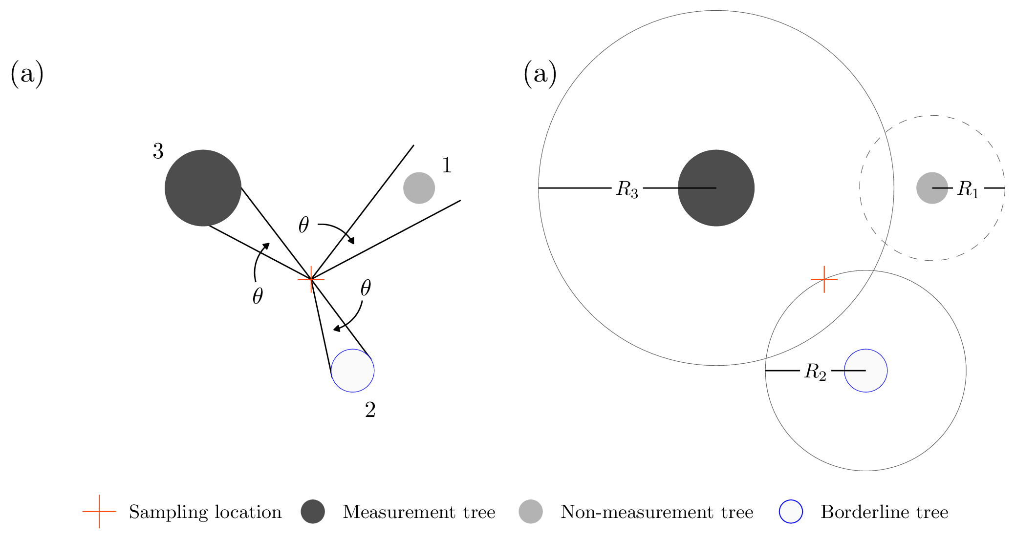
FIGURE 13.8: Point sampling example with three trees around a sampling location. Trees are identified using filled circles with diameter equal to the tree’s DBH. The orange cross indicates the sampling location. (a) Fixed and known angle \(\theta\) is projected from the sampling location and used to identify measurement (3), borderline (2), and non-measurement (1) trees. (b) Unfilled circles identify each tree’s inclusion zone with \(R_1\), \(R_2\) and \(R_3\) being the inclusion zone radius for Trees 1, 2, and 3, respectively. Inclusion zones delineated with solid lines identify measurement and borderline trees. Inclusion zones delineated with dashed lines identify non-measurement trees.
Figure 13.8(a) illustrates a horizontal point sampling measurement tree selection rule. From a sampling location, the forester projects a known and fixed angle \(\theta\) toward each tree’s bole at breast height. Given a tree’s DBH and distance from the sampling location (i.e., the angle’s vertex), the angle may appear:
- wider than the tree bole, in which case the tree is not measured;
- the same width as the tree bole (i.e., the angle’s rays are tangent to the bole), in which case the tree is considered a borderline tree and a measurement determination will take some more effort, as we’ll describe below;
- narrower than the tree bole, in which case the tree is measured.
If we apply this rule to the three trees in Figure 13.8(a), Tree 1 is not measured, Tree 2 is a borderline tree, and Tree 3 is measured. Here again, depending on the inferential objectives, “measured” might imply that you simply tally (i.e., add the tree to a tree count) or take detailed measurements of interest (e.g., DBH, height).
The angle gauge, relascope, and wedge prism are the most common tools used in practice to project the angle \(\theta\) from the sampling location to discern a tree’s measurement status (i.e., is the tree “in” or “out” of the tally). The angle gauge consists of a small piece of metal of known width, held a known distance from the forester’s eye, which is positioned over the sampling location, see, e.g., Fehrmann (2024). The relascope, developed by Walter Bitterlich specifically for point sampling, is a sophisticated and multipurpose tool. The forester sights through the relascope’s eyepiece with their eye positioned over the sampling location. The relascope automatically corrects for slope (see Section 13.4.4) and allows the user to choose among various angles to maximize cruise efficiency (see Section 13.4.3). The wedge prism, introduced by Bruce (1955), is a ground and calibrated prism that refracts light at the desired angle. In contrast to the angle gauge and relascope, where the forester’s eye is the vertex of the angle at the sampling location, the wedge prism itself must be positioned directly over the sampling location. See Burkhart et al. (2018) or similar practical guides to learn how these tools are used.
Let’s begin building some intuition about point sampling by connecting measurement tree selection using an angle with a tree’s inclusion zone as developed in Section 13.3. Recall that under plot sampling, a tree is selected for measurement if its inclusion zone contains a sampling location (see, e.g., Figure 13.1(b)). Also, under plot sampling, all trees have the same inclusion zone area that is equal to the plot area used in the survey.133 Because all trees then have the same inclusion zone, they have equal probability of selection for measurement and, following (13.1), the same tree factor.
Under horizontal point sampling, a tree’s inclusion zone area—and thus its probability of selection—is a function of DBH. As shown in Figure 13.8(b), the circular inclusion zone defined by the tree’s inclusion zone radius (\(R\)) has area proportional to \(\text{DBH}^2\), and therefore proportional to basal area. In other words, larger trees have larger inclusion zones, making them more likely to be selected.
A tree’s inclusion zone radius (\(R\)) is called its limiting distance. This is because if the distance between the sampling location and the tree center is less than or equal to the tree’s limiting distance, then the tree is measured. If the distance between the sampling location and the tree center is greater than the tree’s limiting distance, then the tree is not measured.
This relationship can be seen in Figure 13.8(b). Here, in particular, notice the borderline tree’s limiting distance, \(R_2\), equals the distance between the sampling location and the tree’s center. Figure 13.9 provides a closer look at a borderline tree. At the borderline, the tree is the maximum distance from the sampling location and still measured. Notice in Figure 13.9, if the tree’s DBH is smaller or the tree is farther from the sampling location, the angle would be wider than the tree—hence, it would not qualify for measurement.
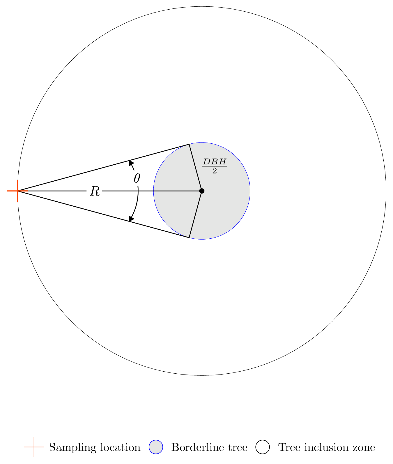
FIGURE 13.9: Horizontal point sampling example of a borderline tree.
When projecting the angle from the sampling location, if there’s uncertainty about a tree’s status (i.e., is it a measurement tree or not), then additional measurements are needed to make a correct determination. This is done by measuring the tree’s DBH, computing its limiting distance, and checking that distance against the distance from the sampling location to the tree’s center.
Even without dense undergrowth or other factors that impair line of sight, it’s often difficult—even for experienced foresters—to identify borderline trees using an angle gauge, prism, or relascope. See, for example, work by Iles and Fall (1988), who assessed professional cruisers’ skill in discerning borderline trees using a wedge prism.134
Incorrect status determination can introduce bias, so it’s worth the extra time to conduct the limiting distance calculation and measurement needed for a correct determination.
For a fixed angle \(\theta\), the relationship between a tree’s DBH and its inclusion zone radius \(R\) is determined by geometry. Specifically, once DBH and \(R\) are expressed in the same length units, their ratio depends only on the chosen angle.
When DBH is measured in inches and \(R\) is measured in feet, converting DBH to feet gives \[\begin{equation} k = \frac{\text{DBH (in)}}{12\,R\text{ (ft)}}. \tag{13.11} \end{equation}\]
Similarly, when DBH is measured in centimeters and \(R\) is measured in meters, converting DBH to meters gives \[\begin{equation} k = \frac{\text{DBH (cm)}}{100\,R\text{ (m)}}. \tag{13.12} \end{equation}\]
In (13.11) and (13.12), the conversion factors (12 or 100) simply rescale DBH into the same length units as \(R\), so the ratio compares two quantities expressed in the same units. Regardless of the measurement system used, this ratio depends only on the chosen angle and can be written as \[\begin{equation} k = 2 \sin\!\left(\frac{\theta}{2}\right). \tag{13.13} \end{equation}\]
Equivalently, the inclusion zone radius can be viewed as a fixed multiple of DBH, with the multiplier determined entirely by the angle used in point sampling.
If \(k\) is known and a tree’s DBH is measured, the corresponding limiting distance can be computed directly. When DBH is measured in inches, the inclusion zone radius in feet is \[\begin{equation} R \text{ (ft)} = \frac{\text{DBH (in)}}{12\,k}. \tag{13.14} \end{equation}\]
Likewise, when DBH is measured in centimeters, the inclusion zone radius in meters is \[\begin{equation} R \text{ (m)}= \frac{\text{DBH (cm)}}{100\,k}. \tag{13.15} \end{equation}\]
The expressions above clarify the geometry of point sampling, but they’re not especially convenient for routine field use. In the next section, we build on these results to develop field-useful expansion factors and point-level summaries for per-unit-area estimation. We then return to the field mechanics in Section 13.4.3 and provide practical formulas for computing the limiting distance \(R\).
13.4.1 Expansion factors and point-level summaries
Recall from Section 13.3.1, the tree factor is the number of trees per unit area a given measurement tree represents. For the \(j\)-th measurement tree, (13.1) defines the tree factor as \[\begin{equation} \text{TF}_j = \frac{\text{unit area}}{\text{inclusion zone area}_j}, \tag{13.16} \end{equation}\] where, depending on your measurement system, the unit area numerator is 43560 (ft\(^2\)/ac) or 10000 (m\(^2\)/ha), and the denominator is the \(j\)-th tree’s inclusion zone area in ft\(^2\) or m\(^2\).135
For horizontal point sampling, the inclusion zone is circular with area equal to \(\pi R_j^2\). Because \(R_j\) is proportional to DBH\(_j\), the tree factor is inversely proportional to DBH\(_j^2\).
Using radius \(R_j\) defined in (13.14), the TF for the English system when DBH is measured in inches is \[\begin{equation*} \text{TF}_j = \frac{43560}{\pi R^2_j} = \frac{43560}{\pi \left(\text{DBH}_j/(12k) \right)^2} = \frac{43560k^2}{ \left(\pi/144\right)\text{DBH}^2_j}, \end{equation*}\] then scaling the numerator and denominator by 1/4 gives us the more revealing and convenient \[\begin{equation} \text{TF}_j = \frac{(1/4)43560k^2}{(1/4)\left(\pi/144\right)\text{DBH}^2_j} = \frac{10890k^2}{0.005454\cdot\text{DBH}^2_j} = \frac{10890k^2}{\text{BA}_j}. \tag{13.17} \end{equation}\] where BA\(_j\) is the \(j\)-th tree’s basal area.
Similarly, using the definition of \(R_j\) from (13.15), the TF for the metric system when DBH is measured in centimeters is \[\begin{equation*} \text{TF}_j = \frac{10000}{\pi R^2_j} = \frac{10000}{\pi \left(\text{DBH}_j/(100k) \right)^2} = \frac{10000k^2}{ \left(\pi/10000\right)\text{DBH}^2_j}, \end{equation*}\] then scaling the numerator and denominator by 1/4 gives us \[\begin{equation} \text{TF}_j = \frac{(1/4)10000k^2}{(1/4)\left(\pi/10000\right)\text{DBH}^2_j} = \frac{2500k^2}{0.00007854\cdot\text{DBH}^2_j} = \frac{2500k^2}{\text{BA}_j}. \tag{13.18} \end{equation}\]
As developed in Section 13.3.1, (13.2) defines the per-unit-area expansion factor for the \(j\)-th tree’s continuous or binary variable measurement (e.g., basal area, volume, biomass, logs, live/dead) as \[\begin{equation} y_j \left(\text{units}/\text{unit area}\right) = y_j \left(\text{units}/\text{tree}\right) \cdot \text{TF}_j \left(\text{trees}/\text{unit area}\right), \tag{13.19} \end{equation}\] where \(y_j\) represents the tree-level variable measurement in the given units.136
It’s instructive to first consider a tree’s basal area expansion, which is called the basal area factor (BAF). Following (13.19) and (13.17), the English system BAF (with units included in parentheses) is \[\begin{align} \text{BAF}_j \left(\text{ft}^2/\text{acre}\right) &= \text{BA}_j \left(\text{ft}^2/\text{tree}\right) \cdot \text{TF}_j \left(\text{trees}/\text{acre}\right)\nonumber\\ &= \cancel{\text{BA}_j} \cdot \left(\frac{10890k^2}{\cancel{\text{BA}_j}}\right)\nonumber\\ &= 10890k^2. \tag{13.20} \end{align}\] and following (13.19) and (13.18), the metric system BAF is \[\begin{align} \text{BAF}_j \left(\text{m}^2/\text{ha}\right) &= \text{BA}_j \left(\text{m}^2/\text{tree}\right) \cdot \text{TF}_j \left(\text{trees}/\text{ha}\right)\nonumber\\ &= \cancel{\text{BA}_j} \cdot \left(\frac{2500k^2}{\cancel{\text{BA}_j}}\right)\nonumber\\ &= 2500k^2. \tag{13.21} \end{align}\]
Notice in (13.20) and (13.21) that BAF depends only on the constant \(k\). As discussed earlier, \(k\) is determined by the angle \(\theta\) used to conduct the cruise.137 Therefore, given \(\theta\), the basal area per unit area represented by each measurement tree is constant. This is a remarkable result! It means that each counted tree represents the same basal area per unit area, regardless of its diameter or its distance from the sample point.
By extension, this means you don’t need to measure a tree’s DBH to determine its contribution to estimating basal area per unit area—all you need to know is whether the tree is a measurement tree or not (i.e., is the tree “in” or “out”)!
For example, say your chosen angle \(\theta\) results in a BAF = 10 (ft\(^2\)/acre). From the result above, we know that each measurement tree (regardless of its DBH) represents 10 ft\(^2\) of basal area per acre. If your chosen angle \(\theta\) results in a BAF = 4 (m\(^2\)/ha), then each measurement tree represents 4 m\(^2\) of basal area per hectare (again, regardless of its DBH).
To expand measurements for variables other than basal area, we follow (13.19), which relies on the tree factor and therefore requires a DBH measurement. Using the results in (13.20) and (13.21) and substituting into (13.17) and (13.18), respectively, the tree factor can be written compactly in terms of the BAF as \[\begin{equation} \text{TF}_j = \frac{\text{BAF}}{\text{BA}_j}. \tag{13.22} \end{equation}\]
For example, say you’re using a BAF = 10 (ft\(^2\)/acre) and the \(j\)-th measurement tree has a DBH of 16 (in) and volume of 45.8 (ft\(^3\)).138 Calculating the \(j\)-th tree’s volume per acre is a two-step process.
First, compute the tree’s tree factor using (13.22) as follows. \[\begin{align*} \text{TF}_j \left(\text{trees}/\text{acre}\right) &= \frac{\text{BAF} \left(\text{ft}^2/\text{acre}\right)}{\text{BA}_j \left(\text{ft}^2/\text{tree}\right)}\\ &= \frac{10}{0.005454\cdot 16^2}\\ &= 7.16217. \end{align*}\]
Then, following (13.19), scale the tree’s volume by its tree factor \[\begin{align*} v_j \left(\text{ft}^3/\text{acre}\right) &= v_j \left(\text{ft}^3/\text{tree}\right)\cdot \text{TF}_j \left(\text{trees}/\text{acre}\right)\\ &= 45.8 \cdot 7.16217 \\ &= 328. \end{align*}\]
So, that one measurement tree represents a volume of 328 ft\(^3\)/acre.
We refer to the process of expanding and summing tree measurements at each sampling location as the point-level summary—the point-sampling analog to the plot-level summary introduced in Section 13.3.1.
For the \(i\)-th sampling location, the point-level summary for basal area per unit area is
\[\begin{equation}
\text{BA}_i = m_i \cdot \text{BAF},
\tag{13.23}
\end{equation}\]
where \(m_i\) is the number of trees counted using the given BAF.
For other variables, the general expression for a point-level summary follows (13.3). For example, trees per acre are given by (13.4) and volume by (13.6). The only difference from plot sampling is that, under point sampling, the tree factor is computed using the basal-area-based form in (13.22).
13.4.2 Sample-based estimates
For \(n\) sampling locations, the corresponding \(n\) per-unit-area point-level summaries of a given variable (see Section 13.4.1) are the sample observations—that is, the \(y_i\) for \(i = 1, 2, \ldots, n\)—used to estimate population parameters via the estimators provided in Section 12.3.
Point sampling follows the same sample-based estimation framework described in Section 12.3, with one exception. As noted at the beginning of Section 13.4, point sampling is unique in that it allows you to match data collection effort with the desired level of inference. The minimum data collection effort is called a continuous tally, meaning a count of measurement trees is kept across the \(n\) sampling locations (no additional information is recorded—not even how many measurement trees were observed at each sampling location).
At the end of a continuous tally cruise, you have the total number of measurement trees \(m\), which is used to compute the mean basal area per-unit-area estimate as \[\begin{equation} \overline{\text{BA}} = \frac{m \cdot \text{BAF}}{n}. \tag{13.24} \end{equation}\]
If you’d like to estimate a confidence interval for mean basal area per unit area, record the number of trees tallied at each sampling location and compute the point-level basal area per unit area (13.23). Recognize these values as your \(y_i\)s and follow the steps in Section 12.3.
Following Section 13.4.1, all variables except basal area require tree factors to compute their point-level summaries.139 Again following the notation in Section 12.3, these \(n\) point-level summaries are your \(y_i\)s, used to compute the sample mean, standard error of the mean, and confidence intervals via (12.15), (12.21), and (12.31), respectively. The same formulas used for plot sampling apply here when point-sampling tree factors are used in place of plot-based ones.
Estimates for totals (e.g., total basal area or volume) in the cruised population follow directly from the per-unit-area estimates as described in Section 12.3.3, with the simple change of replacing the population size \(N\) with the forest area \(A\), expressed in the same units as the per-unit-area means.
Computation of basal area and other parameter estimates under point sampling is illustrated in Section 13.3.6.
13.4.3 Selecting a basal area factor and computing limiting distances
In practice, a horizontal point sampling cruise is described in terms of the BAF, not the angle \(\theta\) that determines the BAF. For example, you might say “the cruise was conducted using a 40 BAF angle gauge (English units),” or perhaps “a 3 BAF wedge prism (metric units).”
While there are no specific rules for selecting a BAF, in practice you should select one that yields an average of 4 to 10 measurement trees per point. BAFs that yield average tree counts outside this range are not wrong—they’re just less efficient.
Given a desired average number of trees per point and a rough estimate for the stand’s basal area per unit area (e.g., obtained via prior experience with similar stands or from a quick preliminary cruise of a few points), select the BAF instrument (e.g., angle gauge or wedge prism) you have that’s closest to the value computed using \[\begin{equation} \frac{\text{stand basal area per unit area}}{\text{desired tree count per point}}. \tag{13.25} \end{equation}\]
For example, say you’d like an average of 7 measurement trees per point. Looking at the stand, you come up with a rough basal area estimate of 150 ft\(^2\)/ac. Then, using (13.25), a reasonable BAF to cruise the stand would be \(150/7 = 21.43\), so select a BAF of 20 (which is a standard instrument size).
Based on the guidance above or an established survey protocol, a single BAF is typically selected for each population in a stand. To keep roughly the same number of measurement trees per point, you might feel tempted to change the BAF from point to point—don’t do this. Changing the BAF from point to point leads to errors and bias, see, e.g., Wensel et al. (1980) and Iles and Wilson (1988).
You can, however, use a different BAF for different populations within a stand, especially if the populations differ substantially in their average DBH and/or basal area. For example, you might choose one BAF for large diameter sawtimber and a separate BAF for small diameter pulpwood. Of course, in such settings, it’s critical to record the BAF used for each population.
Given a BAF, you can find the constant \(k\), the tree’s inclusion zone radius (\(R\)) given its DBH, and the \(\text{R}/\text{DBH}\) ratio called the horizontal distance multiplier (HDM), which is useful for quickly figuring out a tree’s limiting distance. For the English system, with DBH in inches and BAF in ft\(^2\)/ac, these are \[\begin{align} k &= \sqrt{\frac{\text{BAF}}{10890}},\tag{13.26}\\ R \left(\text{ft}\right) &= \frac{\text{DBH}}{12k},\tag{13.27}\\ \text{HDM} \left(\frac{\text{ft}}{\text{in}}\right) &= \frac{R}{\text{DBH}} = \frac{1}{12k}, \tag{13.28} \end{align}\] and for the metric system, with DBH in centimeters and BAF in m\(^2\)/ha, these are \[\begin{align} k &= \sqrt{\frac{\text{BAF}}{2500}},\tag{13.29}\\ R \left(\text{m}\right) &= \frac{\text{DBH}}{100k},\tag{13.30}\\ \text{HDM} \left(\frac{\text{m}}{\text{cm}}\right) &= \frac{R}{\text{DBH}} = \frac{1}{100k}. \tag{13.31} \end{align}\]
The HDM is a convenient value to have with you in the field to determine a tree’s limiting distance. As noted previously, due to competing vegetation or other complicating factors, it might be difficult to discern if a given tree is a measurement tree. In such cases, you’ll need to compare the tree’s limiting distance to the distance between the sampling location and the tree’s center.
Using the HDM, a tree’s limiting distance is computed as \[\begin{equation} R = \text{HDM} \cdot \text{DBH}, \tag{13.32} \end{equation}\] where the HDM has units of distance per unit diameter.
For example, say you’re conducting a cruise using a metric 4 BAF (i.e., \(k\) = 0.04) and the tree in question has a DBH of 30 cm. Then, using (13.32) with the HDM from (13.31), its limiting distance is \[\begin{align*} R &= \text{HDM} \cdot \text{DBH}\\ &= \left(\frac{1}{100 \cdot 0.04}\right) \cdot 30\\ &= 7.5 \text{ m}. \end{align*}\]
Or say you have a borderline tree with a DBH of 18 inches and you’re using an English 10 BAF (i.e., \(k\) = 0.0303). Then, using (13.32) with the HDM from (13.28), its limiting distance is \[\begin{align*} R &= \text{HDM} \cdot \text{DBH}\\ &= \left(\frac{1}{12 \cdot 0.0303}\right) \cdot 18\\ &= 49.5 \text{ ft}. \end{align*}\]
If you’re lucky enough to be working in metric units with DBH in cm and BAF in m\(^2\)/ha, the limiting distance in (13.30) collapses to an easy-to-remember identity, \[\begin{equation} R \left(\text{m}\right) = \frac{\text{DBH (cm)}}{2\sqrt{\text{BAF}}}, \end{equation}\] which is algebraically identical to (13.30) after substituting \(k\) from (13.29). Unfortunately, the English-unit equivalent doesn’t work out as cleanly and isn’t nearly as easy to remember or use in the field.140
While any angle \(\theta\) could be used for a cruise, we generally select ones that provide convenient BAFs to work with (i.e., whole numbers). A few such BAFs and their corresponding angle, constant \(k\), and HDM are provided in Tables 13.6 and 13.7 for the English and metric systems, respectively.141 Such tables are useful to have with you in the field so you can quickly compute a tree’s limiting distance given its DBH and HDM.
| BAF (ft\(^2\)/acre) | Angle \(\theta^\circ\) | Constant \(k\) | HDM (ft/in) |
|---|---|---|---|
| 5 | 1.2277 | 0.02143 | 3.89 |
| 10 | 1.7363 | 0.03030 | 2.75 |
| 15 | 2.1266 | 0.03711 | 2.25 |
| 20 | 2.4556 | 0.04285 | 1.94 |
| 25 | 2.7455 | 0.04791 | 1.74 |
| 30 | 3.0076 | 0.05249 | 1.59 |
| 35 | 3.2486 | 0.05669 | 1.47 |
| 40 | 3.4730 | 0.06061 | 1.38 |
| 50 | 3.8831 | 0.06776 | 1.23 |
| 60 | 4.2539 | 0.07423 | 1.12 |
| BAF (m\(^2\)/ha) | Angle \(\theta^\circ\) | Constant \(k\) | HDM (m/cm) |
|---|---|---|---|
| 1 | 1.1459 | 0.02000 | 0.500 |
| 2 | 1.6206 | 0.02828 | 0.354 |
| 3 | 1.9849 | 0.03464 | 0.289 |
| 4 | 2.2920 | 0.04000 | 0.250 |
| 5 | 2.5626 | 0.04472 | 0.224 |
| 6 | 2.8072 | 0.04899 | 0.204 |
| 7 | 3.0322 | 0.05292 | 0.189 |
| 8 | 3.2416 | 0.05657 | 0.177 |
| 9 | 3.4383 | 0.06000 | 0.167 |
| 10 | 3.6243 | 0.06325 | 0.158 |
13.4.4 Boundary overlap and slope corrections
Like plot sampling, point sampling requires corrections for boundary and slope effects. The need for these corrections is the same as those for plot sampling, namely, selection probability is lower for trees that have their inclusion zone partially outside the forest boundary, and horizontal distance, not slope distance, should be used to determine if a point center falls within a tree’s inclusion zone. The main difference between boundary overlap and slope correction approaches for plot sampling versus horizontal point sampling is that under horizontal point sampling a tree’s inclusion zone is a function of its DBH (whereas under plot sampling, a tree’s inclusion zone and hence selection probability is a function of plot area).
Under horizontal point sampling, if a measurement tree has any portion of its inclusion zone outside the forest boundary, then some approach to correcting the boundary effect should be used. In such cases, either the mirage or walkthrough method introduced in Section 13.3.3 can be applied. An in-depth look at these and other viable correction methods is presented in Kershaw et al. (2016) and Gregoire and Valentine (2008).
As in plot sampling, measurements taken to identify measurement trees are assumed to be on the horizontal plane. The relascope automatically corrects for slope while sighting possible measurement trees, so no additional effort is required to apply the correction. Slope correction using a wedge prism can be done by rotating the prism about the line of sight to match the slope angle along which you are sighting; see USFS (1996) or a similar field methods guide for details.
When using an angle gauge or other devices without a straightforward slope correction, you can convert horizontal limiting distance to slope limiting distance. This calculation is the same as that performed in Section 13.3.3 to compute \(C_1\) and \(C_2\) in Figure 13.5(c), but with plot radius \(R\) replaced by the \(j\)-th tree’s limiting distance \(R_j = \text{HDM} \cdot \text{DBH}_j\), following (13.32).
13.4.5 Illustration
This illustration uses the toy forest population described in Section 13.3.6 and shown in Figure 13.6. Here, point sampling locations are placed at the fixed-area plot centers used previously to illustrate plot sampling. The analysis presented in this section is the point sampling equivalent to the plot sampling analysis.
Recall from the description in Section 13.3.6, these sampling locations were selected using SRS from each stand’s areal sampling frame.
Our aim is to step through the point sampling calculations to estimate per-acre basal area, number of trees, and volume, along with corresponding stand totals. A highly efficient workflow for these and additional estimates is developed in Section 13.6 and applied to data from both stands.
We chose to use an English BAF 20 to select measurement trees at each of the six sampling locations. These sampling locations and their associated measurement trees are shown in Figure 13.10.

FIGURE 13.10: Toy forest inventory dataset comprising two stands and three sampling locations randomly located within each stand. An English BAF 20 was used to identify measurement trees around each sampling location. Each tree’s inclusion zone is added for illustration.
We limit our analysis to overstory tree data in Stand 1. Table 13.8 provides overstory tree measurements for the three Stand 1 points. Notice in Figure 13.10 there are no overstory trees on Point 2 in Stand 1. As mentioned before, it’s critical that absence of trees at a sampling location is included in subsequent estimates—meaning a sampling location with no trees is part of the sample, reflects a characteristic of the population, and needs to be included as a zero when computing population parameter estimates. We include a line for Point 2 in Table 13.8 with zero DBH and volume values to remind us to include these values in subsequent computations.
| Point | DBH (in) | Volume (ft\(^3\)) |
|---|---|---|
| 1 | 10.7 | 17.9 |
| 1 | 9.8 | 14.5 |
| 1 | 11.3 | 17.8 |
| 2 | 0.0 | 0.0 |
| 3 | 13.1 | 28.9 |
| 3 | 14.8 | 33.6 |
| 3 | 15.4 | 36.6 |
Let’s begin by assuming this was a continuous tally cruise, which, recall from Section 13.4.2, means the forester only kept track of the total number of measurement trees, \(m\), across the entire cruise. Looking at Figure 13.10, or by counting the non-zero rows in Table 13.8, we can see there were \(m = 6\) measurement trees across the \(n = 3\) sampling locations in Stand 1. Then, following (13.24), the estimate for basal area per acre is \[\begin{equation*} \overline{\text{BA}} = \frac{m \cdot \text{BAF}}{n} = \frac{6 \cdot 20}{3} = 40 \left(\text{ft}^2/\text{acre}\right). \end{equation*}\]
Given Stand 1’s area is \(A\) = 0.64 acres, and following (12.22), with the slight modification of replacing \(N\) with \(A\), the continuous tally estimate for total basal area for Stand 1 is \(A\cdot \overline{\text{BA}} = A(m\cdot \text{BAF})/n = 0.64\cdot 40 = 26\) (ft\(^2\)).
If you want a standard error to accompany the mean or total basal area estimates, then keep track of how many measurement trees were counted at each sampling location and compute the basal area per acre point-summaries as illustrated below.
Just like estimation using plot sampling data illustrated in Section 13.3.6, we divide the estimation process into two steps. First, compute point-level summaries for each variable (see the end of Section 13.4.1). The point-level summaries comprise each point’s expanded and summarized tree measurements expressed on a per-unit-area basis (these are the sample observations). Second, use the point-level summaries to compute the desired population parameter estimates (see Section 13.4.2).
Using the measurement tree counts at each sampling location, \(m_1\) = 3, \(m_2\) = 0, and \(m_3\) = 3, and following (13.23), point-level basal area per acre summaries are \[\begin{alignat*}{2} &\text{Point 1:}&&\; m_1\!\cdot\!\text{BAF} = 3\!\cdot\!20 = 60 \left(\text{ft}^2/\text{ac}\right),\\ &\text{Point 2:}&&\; m_2\!\cdot\!\text{BAF} = 0\!\cdot\!20 = 0 \left(\text{ft}^2/\text{ac}\right),\\ &\text{Point 3:}&&\; m_3\!\cdot\!\text{BAF} = 3\!\cdot\!20 = 60 \left(\text{ft}^2/\text{ac}\right). \end{alignat*}\]
To compute the point-level summaries for all other variables, we include each measurement tree’s tree factor from (13.22). Using (13.19) and (13.22), and referring to Table 13.8 to compute each measurement tree’s basal area from its DBH, the point-level estimate of trees per acre are \[\begin{alignat*}{2} \text{Point 1:} &\; \sum^3_{j=1}\text{TF}_j = \sum^3_{j=1}\frac{\text{BAF}}{c\cdot\text{DBH}^2_j} &&= \frac{20}{c\cdot 10.7^2} + \frac{20}{c\cdot 9.8^2} + \frac{20}{c\cdot 11.3^2}\\ & &&= 32.02929 + 38.18235 + 28.71825\\ & &&= 98.92989 \left(\text{trees}/\text{ac}\right),\\[1pt] \text{Point 2:} & &&= 0 \left(\text{trees}/\text{ac}\right),\\[1pt] \text{Point 3:} &\; \sum^3_{j=1}\text{TF}_j = \sum^3_{j=1}\frac{\text{BAF}}{c\cdot\text{DBH}^2_j} &&= \frac{20}{c\cdot 13.1^2} + \frac{20}{c\cdot 14.8^2} + \frac{20}{c\cdot 15.4^2}\\ & &&= 21.36841 + 16.74139 + 15.46228\\ & &&= 53.57208 \left(\text{trees}/\text{ac}\right), \end{alignat*}\] where \(c = 0.005454\).142
Using (13.19) and the volume measurements in Table 13.8 along with the tree factors computed above, point-level volume per acre are \[\begin{alignat*}{2} \text{Point 1:} &\; \sum^3_{j=1}v_j\cdot \text{TF}_j &&= 17.9\cdot32.02929 + 14.5\cdot38.18235 + 17.8\cdot28.71825\\ & &&= 573.32428 + 553.64415 + 511.18485\\ & &&= 1638.15329 \left(\text{ft}^3/\text{ac}\right),\\[1pt] \text{Point 2:} & &&= 0 \left(\text{ft}^3/\text{ac}\right),\\[1pt] \text{Point 3:} &\; \sum^3_{j=1}v_j\cdot \text{TF}_j &&= 28.9\cdot21.36841 + 33.6\cdot16.74139 + 36.6\cdot15.46228\\ & &&= 617.54714 + 562.5106 + 565.9193\\ & &&= 1745.97704 \left(\text{ft}^3/\text{ac}\right), \end{alignat*}\] where \(v_j\) is the \(j\)-th tree’s volume.
For reference, we collected the point-level summaries of basal area, number of trees, and volume per acre computed above into Table 13.9. Given the \(n\) = 3 sample observations in Table 13.9, you’re back in familiar territory for computing SRS means, standard deviations, standard errors, and confidence intervals covered in Sections 12.3 and 13.4.2.
| Point | Basal area (ft\(^2\)/ac) | Trees/ac | Volume (ft\(^3\)/ac) |
|---|---|---|---|
| 1 | 60 | 98.9299 | 1638.1533 |
| 2 | 0 | 0 | 0 |
| 3 | 60 | 53.5721 | 1745.977 |
The code below computes each variable’s mean (12.15), standard error of the mean (12.21), and 90% confidence interval. Again, as discussed in Section 13.2.1, when we select sampling locations using an areal sampling frame, we don’t apply the FPC when calculating the standard error of the mean.
n <- 3 # Sample size.

t <- qt(p = 1 - 0.1 / 2, df = n - 1) # t-value for 90% CI.

# Basal area per acre.
ba_i <- c(60, 0, 60)
ba_bar <- mean(ba_i)
s_ba_bar <- sd(ba_i) / sqrt(n)
ci_ba <- c(ba_bar - t*s_ba_bar,
           ba_bar + t * s_ba_bar)

ba_bar #Mean basal area per acre.
#> [1] 40#> [1] -18.4 98.4# Trees per acre.
trees_i <- c(98.9299, 0, 53.5721)
trees_bar <- mean(trees_i)
s_trees_bar <- sd(trees_i) / sqrt(n)
ci_trees <- c(trees_bar - t * s_trees_bar,
trees_bar + t * s_trees_bar)
trees_bar #Mean number of trees per acre.#> [1] 50.834#> [1] -32.652 134.320# Volume per acre.
vol_i <- c(1638.1533, 0, 1745.977)
vol_bar <- mean(vol_i)
s_vol_bar <- sd(vol_i) / sqrt(n)
ci_vol <- c(vol_bar - t * s_vol_bar,
vol_bar + t * s_vol_bar)
vol_bar #Mean volume per acre.#> [1] 1128#> [1] -521.4 2777.5The mean and associated confidence interval computed in the code above are collected into Table 13.10.
| \(\bar{y}\) | 90% CI | |
|---|---|---|
| Trees/ac | 50.834 | (-32.652, 134.32) |
| Basal area (ft\(^2\)/ac) | 40.000 | (-18.4, 98.4) |
| Volume (ft\(^3\)/ac) | 1128.043 | (-521.398, 2777.485) |
Stand 1 total and associated confidence interval for each variable can be computed using (12.22) and (12.25). These estimators for the total are modified by replacing population size \(N\) with stand area in acres \(A\) = 0.64. Total estimates are given in Table 13.11. Importantly, notice that obtaining totals and associated confidence intervals is as easy as scaling mean per-acre estimates given in Table 13.10 by \(A\).
| \(\hat{t}\) | 90% CI | |
|---|---|---|
| Trees | 32.534 | (-20.898, 85.965) |
| Basal area (ft\(^2\)) | 25.600 | (-11.776, 62.976) |
| Volume (ft\(^3\)) | 721.948 | (-333.695, 1777.59) |
Take a moment to compare point and plot sampling estimates in Tables 13.4 and 13.5 versus Tables 13.10 and 13.11. We expect some differences because different rules are used to select measurement trees, and tree expansion factors are computed differently. In practice, point and plot sampling will yield different estimates for any given single sample. However, both are unbiased methods, and hence, over repeated sampling, we’d expect their estimates to agree on average.
As in the plot sampling example, the confidence intervals include negative values for strictly positive parameters. This occurs here due to small sample size and large variance, and reflects the limitations of symmetric approximation methods. See Section 13.5 for further discussion.
13.4.6 Per-unit-area estimates without measuring DBH
A key advantage to horizontal point sampling is that basal area per unit area can be estimated without measuring DBH. However, as we saw in the preceding sections, the tree factor (and hence DBH measurement) is needed to obtain estimates for other parameters. There is an approach to obtaining per-unit-area estimates using variables that scale linearly with basal area across some measure of tree height, without measuring DBH. In such cases, a tree height measurement replaces the DBH measurement. This approach is practical when a measure of tree height can be obtained more easily than DBH.
Depending on the variable of interest, the tree height measurement can take a variety of forms, e.g., total height, height to a given stem diameter, or stem segment length such as a 16 ft sawlog or 2 m bolt. The approach described in this section is often referred to as tally by height.
Variables associated with tree volume and weight often scale linearly with basal area across height. In some cases, such relationships are well described by the constant form factor equation \[\begin{equation} y_j = \alpha \text{DBH}^2_j h_j, \tag{13.33} \end{equation}\] where, for the \(j\)-th tree, \(y_j\) is the variable of interest, \(\alpha\) is a parameter to be estimated, and \(h_j\) is some measure of height.
Dividing both sides of (13.33) by basal area yields the following \[\begin{align} \frac{y_j}{\text{BA}_j} &= \frac{\alpha \text{DBH}^2_j h_j}{\text{BA}_j}\nonumber\\ &= \frac{\alpha \cancel{\text{DBH}^2_j} h_j}{c\cancel{\text{DBH}^2_j}}\nonumber\\ &= \beta h_j, \tag{13.34} \end{align}\] where \(c\) is the basal area constant and \(\beta = \alpha/c\). Importantly, notice in (13.34) the \(y_j\) to \(\text{BA}_j\) ratio (left side) is a function of height \(\beta h_j\) (right side). This means that if we have a tree’s height measurement (\(h_j\)) and a suitable value for \(\beta\), then we can estimate the \(y_j\) to \(\text{BA}_j\) ratio. In the forestry literature, if \(y_j\) is a measure of volume, then the volume-to-basal-area ratio (i.e., \(y_j/\text{BA}_j\)) is called VBAR\(_j\) (pronounced “v bar”). Similarly, if \(y_j\) is a measure of weight, the ratio is called WBAR\(_j\) (pronounced “w bar”).
We typically want a per-unit-area estimate for \(y_j\) (i.e., \(y_j\) value expanded to per-acre or per-hectare basis), not the \(y_j\) to \(\text{BA}_j\) ratio per-unit-area. To get the desired per-unit-area estimate, multiplying both sides of (13.34) by the BAF yields the following \[\begin{equation} \frac{\text{BAF}\cdot y_j}{\text{BA}_j} = \text{BAF}\beta h_j, \end{equation}\] which can be expressed as \[\begin{equation} y_j \cdot \text{TF}_j = \text{BAF}\beta h_j, \tag{13.35} \end{equation}\] because the tree expansion factor \(\text{TF}_j = \text{BAF}/\text{BA}_j\) (13.22). Hence, (13.35) shows you can obtain the desired per-unit-area estimate for \(y_j\) (i.e., \(y_j \cdot \text{TF}_j\)) given your chosen BAF, a value for \(\beta\), and a tree height measurement (via \(\text{BAF}\beta h_j\)).
For example, say you’re interested in estimating lumber volume in board-feet (bd ft) using the International 1/4 log rule per acre.143 Based on prior information, you choose a constant form factor equation that measures trees in 16 ft logs. Following (13.35), the \(j\)-th measurement tree’s volume per acre is \[\begin{align} v_j \cdot \text{TF}_j \left(\frac{\text{bd ft}}{\text{acre}}\right) &= \text{BAF} \left(\frac{\text{ft}^2}{\text{acre}}\right)\cdot \beta \left(\frac{\frac{\text{bd ft}}{\text{ft}^2}}{\text{logs}}\right)\cdot h_j \left(\text{logs}\right)\nonumber\\ &= \text{BAF} \left(\frac{\text{ft}^2}{\text{acre}}\right)\cdot \beta h_j \left(\frac{\text{bd ft}}{\text{ft}^2}\right)\nonumber\\ &= \text{BAF} \beta h_j \tag{13.36} \end{align}\]
Say you’re given a \(\beta\) value of 55.41 and you conduct your cruise using an English 20 BAF prism. If the \(j\)-th measurement tree held \(h_j = 2\) (16 ft logs), then following (13.36), that tree represents \(\text{BAF} \beta h_j = 20 \cdot 55.41 \cdot 2 = 2216.4\) bd ft per acre.
As described toward the end of Section 13.4.1, the area-expanded estimate \(y_j \cdot \text{TF}_j\) is combined with those from other measurement trees at a given sampling location to arrive at the point-level summary.
Continuing our example, say there are \(m_i\) measurement trees at the \(i\)-th sampling location and the total number of logs for those trees was \(h_i = \sum^{m_i}_{j = 1} h_{i,j}\). The point-level summary for the \(i\)-th location equals \(v_i \cdot \text{TF}_i = 20 \cdot 55.41 \cdot h_i\). Point-level summaries from \(n\) sampling locations are used to estimate population parameters following steps in Section 13.4.2.
The tally by height approach produces reasonable estimates only if the following conditions are met.
- The linear relationship described in (13.34) holds across the range of anticipated height values.
- Variability in the variable (e.g., volume or weight) to basal area ratio is small for a given height increment.
The linear relationship, described by the slope parameter \(\beta\), is highly dependent on species, local environment, and stand characteristics, e.g., age, density, disturbance history. As a result, a \(\beta\) estimated for one species and stand might not be appropriate for a different species or stand.
Let’s take a closer look at how one might estimate \(\beta\) for a given variable, species, and geographic region. Table 13.12 holds balsam fir (Abies balsamea) volume values published by Young (1957). Table entries, broken out by DBH and height class, summarize volume (ft\(^3\)) measurements taken on 270 trees in central Maine.
| DBH (in) | 30 | 40 | 50 | 60 | 70 |
|---|---|---|---|---|---|
| 5 | 1.40 | 1.91 | 2.45 | ||
| 6 | 2.14 | 2.83 | 3.60 | ||
| 7 | 3.07 | 4.09 | 5.00 | 6.26 | |
| 8 | 4.20 | 5.60 | 6.82 | 8.42 | 9.85 |
| 9 | 5.56 | 7.18 | 8.77 | 10.75 | 12.53 |
| 10 | 8.90 | 10.90 | 13.33 | 15.56 | |
| 11 | 10.64 | 13.22 | 16.05 | 18.77 | |
| 12 | 15.53 | 18.78 | 21.83 | ||
| 13 | 18.12 | 21.75 | 25.27 | ||
| 14 | 20.87 | 24.76 | 28.66 | ||
| 15 | 28.18 | 32.20 |
Table 13.13 holds volume-to-basal-area ratios (VBARs) computed using volume and DBH from Table 13.12. For example, the VBAR in Table 13.13 for a 5 inch DBH and 30 foot tree is 10.27 (ft\(^3\)/ft\(^{2}\)), which, working from values in Table 13.12, is 1.40 (ft\(^3\)) divided by \(c \cdot \text{DBH}^2 = 0.005454 \cdot 5^2 = 0.13635\) (ft\(^2\)).144
| DBH (in) | 30 | 40 | 50 | 60 | 70 |
|---|---|---|---|---|---|
| 5 | 10.27 | 14.01 | 17.97 | ||
| 6 | 10.90 | 14.41 | 18.34 | ||
| 7 | 11.49 | 15.30 | 18.71 | 23.42 | |
| 8 | 12.03 | 16.04 | 19.54 | 24.12 | 28.22 |
| 9 | 12.59 | 16.25 | 19.85 | 24.33 | 28.36 |
| 10 | 16.32 | 19.99 | 24.44 | 28.53 | |
| 11 | 16.12 | 20.03 | 24.32 | 28.44 | |
| 12 | 19.77 | 23.91 | 27.80 | ||
| 13 | 19.66 | 23.60 | 27.42 | ||
| 14 | 19.52 | 23.16 | 26.81 | ||
| 15 | 22.96 | 26.24 |
Table 13.13 cell color makes apparent the small variability among VBARs within a given 10 ft height class. Recall this is one data characteristic needed for the tally by height approach to produce reasonable estimates. The other data characteristic is a linear relationship between VBARs across the range of anticipated height values. Figure 13.11 is a scatter plot created from values in Table 13.13. Imposed on the scatter plot is a “best fit” line with intercept fixed at zero and slope \(\beta\).145 Visual inspection of the point scatter and line suggests a strong linear relationship exists across the height classes. The line’s slope \(\beta\) = 0.393 is used in (13.35) and would yield reasonable tally by height volume per-acre estimates for balsam fir in central Maine.

FIGURE 13.11: Scatter plot of Table 13.13 volume-to-basal-area ratios (VBARs) for balsam fir (Abies balsamea) in central Maine. Point colors correspond to VBAR values in Table 13.13.
13.5 Negative confidence interval bounds and defensive coding
In the illustrations for plot and point sampling (Sections 13.3.6 and 13.4.5, respectively) we pointed out that the 90% confidence intervals for some estimates include negative lower bounds. This can happen when using normal approximations to construct confidence intervals for forest parameters like stem density, basal area, or volume—quantities that are strictly positive. When sample sizes are small or variances are large, as in the toy example here (\(n = 3\)), confidence intervals may extend into the negative range, even though such values are not meaningful for parameters that must be zero or greater.
While this issue may arise in small-sample or high-variance settings, it’s uncommon in operational forest inventory, where sample sizes are typically larger and variability lower. Still, when it does occur, it’s worth recognizing and addressing. A simple option is to truncate the lower bound at zero, though this can distort the stated confidence level. More generally, if the goal is to better handle non-normal sampling distributions or enforce constraints that reflect the parameter’s support, you may need to look beyond design-based inference and consider other approaches—such as model-assisted or model-based methods—where distributional assumptions are built directly into the estimator (see, e.g., Särndal et al. (1992) and Rao and Molina (2015)).
Encounters with unexpected results—like a confidence interval suggesting an impossible value—are not just statistical curiosities. They’re reminders to pause and think carefully about your workflow. This kind of deliberate checking falls under the broader practice of defensive programming—a mindset that assumes things can go wrong and encourages coding habits that prevent silent failures. In statistical computing, this means checking inputs, intermediate results, and final outputs for consistency with both the math and the context. For example, a negative lower confidence bound for a strictly positive parameter isn’t just a numerical oddity—it’s a cue to revisit your data, assumptions, estimators, and code to make sure everything aligns. Thoughtful debugging isn’t an afterthought; it’s an essential part of reproducible and trustworthy data science.
Brian W. Kernighan, a pioneering computer scientist best known for co-authoring The C Programming Language and for his work on Unix at Bell Labs, put it succinctly:
Everyone knows that debugging is twice as hard as writing a program in the first place. So if you’re as clever as you can be when you write it, how will you ever debug it?
— Brian W. Kernighan
Debugging is indeed difficult—especially in analysis workflows where silent failures can lead to plausible but incorrect results. One of the most effective strategies is to pair deliberate reasoning with simple tools that make your workflow more transparent. Again, Kernighan’s advice remains timeless:
The most effective debugging tool is still careful thought, coupled with judiciously placed print statements.
— Brian W. Kernighan
13.6 Workflows for forest inventory data
13.6.1 Plot sampling illustration
Here we use tidyverse functions to repeat and expand on the analysis presented in Section 13.3.6. Recall that the analysis used a toy dataset to illustrate plot sampling estimation methods. As described in Section 13.3.6 and illustrated in Figure 13.7, the dataset comprises two stands, each with three overstory and nested regeneration plots. The overstory and regeneration plots are circular fixed areas with 24 ft and 6.8 ft radii, respectively. Plot sampling locations were selected using SRS from each stand’s areal sampling frame and serve as the overstory plot centers.
The code below reads in the data collected on the inventory plots and prints its structure.
#> Rows: 30
#> Columns: 8
#> $ stand_id        <dbl> 1, 1, 1, 1, 1, 1, 1, 1, 1, 1, 1, 1…
#> $ plot_id         <dbl> 1, 1, 1, 1, 1, 2, 2, 2, 3, 3, 3, 3…
#> $ tree_type       <chr> "Overstory", "Overstory", "Oversto…
#> $ tree_count      <dbl> 1, 1, 1, 1, 1, 0, 1, 1, 1, 1, 1, 2…
#> $ scientific_name <chr> "Abies balsamea", "Pinus strobus",…
#> $ DBH_in          <dbl> 11.3, 9.8, 10.7, NA, NA, 0.0, NA, …
#> $ height_ft       <dbl> 60.2, 61.1, 63.6, NA, NA, 0.0, NA,…
#> $ vol_cu_ft       <dbl> 17.8, 14.5, 17.9, NA, NA, 0.0, NA,…
Column definitions for stands are as follows.
stand_idstand number within which the plot falls, takes values 1 or 2.plot_idplot number within the stand on which the measurements are recorded.tree_typetype of plot on which the tree was measured, takes valuesOverstoryorRegen.tree_countnumber of trees measured on the plot that have the same values for the next four columns, or zero if no trees occurred on the plot.speciesmeasurement tree species.DBH_inmeasurement tree DBH (in).height_ftmeasurement tree height (ft).vol_cu_ftmeasurement tree volume (ft\(^3\)).
There are a few things to notice about these data (run stands %>% print(n = nrow(.)) to see all the data).
- Plot numbers are unique within the stand, meaning both stand and plot must be specified to identify a plot’s set of trees.
- Because we’re only interested in regeneration density by species for this survey, trees on regeneration plots have
NAvalues for their DBH, height, and volume. - As you might have noticed in Figure 13.7, there are no overstory trees on Plot 2 in Stand 1. It’s critical that the absence of trees at a sampling location be included in subsequent estimates—meaning a plot with no trees is part of the sample, reflects a characteristic of the population, and needs to be included as a zero when computing population parameter estimates. Here, we chose to record plots with no trees using a
tree_countvalue of zero. - In addition to tracking plots with zero measurement trees, the
tree_countcolumn records the number of trees on a given plot that share the same species and measurements on other variables. This allows each row in the data file to represent more than one tree. It’s common in timber cruises to record DBH and number of logs to the nearest whole number, in which case there are often several overstory trees on a plot with counts greater than one. Also, including a tree count variable allows us to accommodate double-count boundary trees identified using the mirage or walkthrough method described in Section 13.3.3, minimize the number of data rows needed to record the inventory data, and build an efficient analysis workflow.
To compare results with those presented in Section 13.3.6, we derive estimates for overstory per-acre number of trees, basal area, and volume, along with corresponding stand totals. Also, following Section 13.3.6, the estimation process is done in two steps. Step 1, compute plot-level summaries for each variable. The plot-level summaries comprise each plot’s expanded and summarized tree measurements expressed on a per-unit-area basis. Step 2, use the plot-level summaries from Step 1 to compute the desired population parameter estimates.
The first bit of code below makes a new tibble (o_stands) that includes only rows corresponding to overstory tree measurements and a column (TF) that holds their tree factors. As you’ll see in the subsequent piped workflow, it’s convenient to have a tree factor column pre-computed.146 The tree factor equation used in mutate() follows (13.1).
The second bit of code below creates the plot-level per-acre summary for each variable. Importantly, notice we group by stand_id and plot_id so the subsequent summarize() works on trees in each plot—yielding plot-level summaries. The equations used to compute these plot-level summaries within summarize() follow (13.2) and parallel steps in Section 13.3.6. The only difference here is we scale by tree_count to accommodate how the data were recorded (i.e., tree_count records the number of trees with common species, DBH, height, and volume, or the absence of trees on a plot).
# Select overstory trees and add a TF trees/ac column.
o_stands <- stands %>%
  filter(tree_type == "Overstory") %>%
  mutate(TF = 43560 / (pi * 24^2))

# Step 1, compute per-unit-area plot-level summaries.
c <- pi / (144 * 4) # Basal area constant.

plot_summary <- o_stands %>%
  group_by(stand_id, plot_id) %>%
  summarize(trees_i = sum(tree_count * TF),
            ba_i = sum(tree_count * TF * c * DBH_in^2),
            vol_i = sum(tree_count * TF * vol_cu_ft),
            .groups = "drop_last")

plot_summary
#> # A tibble: 6 × 5
#> # Groups: stand_id [2]
#> stand_id plot_id trees_i ba_i vol_i
#> <dbl> <dbl> <dbl> <dbl> <dbl>
#> 1 1 1 72.2 44.4 1208.
#> 2 1 2 0 0 0
#> 3 1 3 72.2 82.4 2386.
#> 4 2 1 72.2 22.2 479.
#> 5 2 2 72.2 28.9 669.
#> 6 2 3 96.3 33.2 749.The plot_summary values for stand_id 1 match those computed in Section 13.3.6 and displayed in Table 13.3.
Importantly, the summarize() in Step 1 above uses the default .groups = "drop_last" rule, so the resulting plot_summary is grouped by stand_id and is ready to be summarized by stand in Step 2 below.
The code below uses the plot-level summaries (plot_summary) to compute estimates for the population parameters.147 In the summarize(), we first compute stand-specific sample size n and \(\tval\)-value for a 90% confidence interval to parallel the analysis in Section 13.3.6, then mean, standard error, and confidence interval bounds for the three variables (trees_i, ba_i, and vol_i). The resulting per-acre estimates and associated confidence intervals for Stand 1 and 2 are held in stand_estimates row 1 and 2, respectively. Below, we pass stand_estimates to glimpse() so the output fits on the page. From this printed output, you can see stand_id 1 column values match those computed in Section 13.3.6 and presented in Table 13.4. Values in the second column printed below correspond to estimates for stand_id 2.
# Step 2, compute per-unit-area estimates for each stand.
stand_estimates <- plot_summary %>%
  summarize(n = n(), # Sample size.
            t = qt(p = 1 - 0.1 / 2, df = n - 1), # t-value for 90% CI.
            trees_bar = mean(trees_i),
            s_trees_bar = sd(trees_i) / sqrt(n),
            ci_lower_trees = trees_bar - t * s_trees_bar,
            ci_upper_trees = trees_bar + t * s_trees_bar,
            ba_bar = mean(ba_i),
            s_ba_bar = sd(ba_i) / sqrt(n),
            ci_lower_ba = ba_bar - t * s_ba_bar,
            ci_upper_ba = ba_bar + t * s_ba_bar,
            vol_bar = mean(vol_i),
            s_vol_bar = sd(vol_i) / sqrt(n),
            ci_lower_vol = vol_bar - t * s_vol_bar,
            ci_upper_vol = vol_bar + t * s_vol_bar)

stand_estimates %>% glimpse()
#> Rows: 2
#> Columns: 15
#> $ stand_id <dbl> 1, 2
#> $ n <int> 3, 3
#> $ t <dbl> 2.92, 2.92
#> $ trees_bar <dbl> 48.144, 80.241
#> $ s_trees_bar <dbl> 24.0722, 8.0241
#> $ ci_lower_trees <dbl> -22.146, 56.810
#> $ ci_upper_trees <dbl> 118.43, 103.67
#> $ ba_bar <dbl> 42.278, 28.110
#> $ s_ba_bar <dbl> 23.8185, 3.2139
#> $ ci_lower_ba <dbl> -27.272, 18.725
#> $ ci_upper_ba <dbl> 111.827, 37.494
#> $ vol_bar <dbl> 1198.0, 632.3
#> $ s_vol_bar <dbl> 688.670, 79.987
#> $ ci_lower_vol <dbl> -812.91, 398.73
#> $ ci_upper_vol <dbl> 3208.90, 865.86The workflow above is good, but let’s make it less verbose and more flexible. Notice in the summarize() above, the same operations are applied to each variable. Specifically, say trees_i, ba_i, or vol_i is generically represented with y, then the operations to compute the mean and its standard error are mean(y) and sd(y)/sqrt(n), respectively. As illustrated in the code below, application of these common operations to each variable allows us to use across() (Section 8.11) to simplify the code.
In the summarize() below, the call to across() computes the mean, standard error of the mean, and confidence bounds for each variable. To simplify the code, we use a custom function se() to compute the standard error of the mean for each variable (writing custom functions is covered in Chapter 6). The call to across() also uses the anonymous function lambda syntax introduced in Section 8.11, that is, the tilde ~ and .x syntax.
The .names argument in across() controls how the new column names are formed. Within the string, {.col} is replaced by the name of the input column and {.fn} is replaced by the name of the applied function. This lets you define exactly how the output variable names should look. In this example, we use a small string substitution sub('_i$', '', .col) to remove the trailing _i from each input variable name before appending the function name. As a result, column names like trees_i, ba_i, and vol_i become trees, ba, and vol, producing cleaner and more readable outputs such as y_bar_trees, s_y_bar_trees, and ci_upper_trees.
# Function to compute the standard error of the mean.
se <- function(y, n){
  sd(y) / sqrt(n)
}

# Alternative Step 2, compute per-unit-area estimates for each stand.
plot_summary %>%
 summarize(
   n = n(), # Sample size.
   t = qt(p = 1 - 0.1 / 2, df = n - 1), # t-value for 90% CI.
   across(.cols = c("trees_i", "ba_i", "vol_i"),
          .fns = list(y_bar = mean,
                      s_y_bar = ~ se(.x, n),
                      ci_lower = ~ mean(.x) - t * se(.x, n),
                      ci_upper = ~ mean(.x) + t * se(.x, n)
                      ),
          .names = "{.fn}_{sub('_i$', '', .col)}")) %>%
     glimpse()
#> Rows: 2
#> Columns: 15
#> $ stand_id <dbl> 1, 2
#> $ n <int> 3, 3
#> $ t <dbl> 2.92, 2.92
#> $ y_bar_trees <dbl> 48.144, 80.241
#> $ s_y_bar_trees <dbl> 24.0722, 8.0241
#> $ ci_lower_trees <dbl> -22.146, 56.810
#> $ ci_upper_trees <dbl> 118.43, 103.67
#> $ y_bar_ba <dbl> 42.278, 28.110
#> $ s_y_bar_ba <dbl> 23.8185, 3.2139
#> $ ci_lower_ba <dbl> -27.272, 18.725
#> $ ci_upper_ba <dbl> 111.827, 37.494
#> $ y_bar_vol <dbl> 1198.0, 632.3
#> $ s_y_bar_vol <dbl> 688.670, 79.987
#> $ ci_lower_vol <dbl> -812.91, 398.73
#> $ ci_upper_vol <dbl> 3208.90, 865.86We finish this section by extending our workflow to estimate parameters for both overstory and regeneration populations. Importantly, the only thing we need to do is include those trees measured on the smaller regeneration plots (i.e., 6.8 ft radius plots) and their associated tree factors; the rest of the workflow stays pretty much the same.
Recall the tree_type column indicates if a tree was measured on the overstory or regeneration plot using Overstory and Regen. values, respectively. Using (13.1), the code below illustrates if_else() and case_when() within mutate() to add tree_type specific tree factors (TF) to stands. Both approaches result in the same TF; we include both simply for demonstration. The last line of code below is included to double check that tree factors are correctly assigned to each tree type (again, following from Section 13.3.1, one overstory tree represents approximately 24.1 trees per acre and one regeneration tree represents 300 trees per acre).
# Add TF trees/ac column for each tree type (plot size).
stands <- stands %>% mutate(TF = if_else(tree_type == "Overstory",
                                         43560 / (pi * 24^2),
                                         43560 / (pi * 6.8^2))
                            )

# Or equivalently.
stands <- stands %>%
 mutate(TF = case_when(tree_type == "Overstory" ~ 43560 / (pi * 24^2),
                       tree_type == "Regen." ~ 43560 / (pi * 6.8^2))
         )

# Double check TF is correct for each tree type (plot size).
stands %>% group_by(tree_type) %>% distinct(TF)
#> # A tibble: 2 × 2
#> # Groups: tree_type [2]
#> tree_type TF
#> <chr> <dbl>
#> 1 Overstory 24.1
#> 2 Regen. 300.Now, given our tree_type-specific tree factor in TF, we can move to the familiar two-step estimation process. Step 1, create plot-level summaries. Step 2, summarize at the stand level using the plot-level summary. The code below is identical to what we used for the overstory-only analysis above, except we add tree_type as the first grouping column to produce separate overstory and regeneration plot summaries.
# Step 1, compute per-unit-area plot-level summaries.
c <- pi / (144 * 4) # Basal area constant.

plot_summary <- stands %>%
  group_by(tree_type, stand_id, plot_id) %>%
  summarize(trees_i = sum(tree_count * TF),
            ba_i = sum(tree_count * TF * c * DBH_in^2),
            vol_i = sum(tree_count * TF * vol_cu_ft),
            .groups = "drop_last") # Keep groups tree_type and stand_id.

plot_summary
#> # A tibble: 12 × 6
#> # Groups: tree_type, stand_id [4]
#> tree_type stand_id plot_id trees_i ba_i vol_i
#> <chr> <dbl> <dbl> <dbl> <dbl> <dbl>
#> 1 Overstory 1 1 72.2 44.4 1208.
#> 2 Overstory 1 2 0 0 0
#> 3 Overstory 1 3 72.2 82.4 2386.
#> 4 Overstory 2 1 72.2 22.2 479.
#> 5 Overstory 2 2 72.2 28.9 669.
#> 6 Overstory 2 3 96.3 33.2 749.
#> 7 Regen. 1 1 600. NA NA
#> 8 Regen. 1 2 600. NA NA
#> 9 Regen. 1 3 1199. NA NA
#> 10 Regen. 2 1 900. NA NA
#> 11 Regen. 2 2 900. NA NA
#> 12 Regen. 2 3 1199. NA NARecall DBH and volume were not recorded for trees measured on regeneration plots, hence the NA values in the regeneration rows for ba_i and vol_i.
Stand-level estimates can now be generated by passing plot_summary to summarize(). We could use the previous overstory analysis code unchanged; however, for brevity, below we opt to compute only stand density estimates using trees_i for the regeneration and overstory populations.
# Step 2, compute per-unit-area estimates.
stand_estimates <- plot_summary %>%
  summarize(n = n(), # Sample size.
            t = qt(p = 1 - 0.1 / 2, df = n - 1), # t-value for 90% CI.
            trees_bar = mean(trees_i),
            s_trees_bar = sd(trees_i) / sqrt(n),
            ci_lower = trees_bar - t * s_trees_bar,
            ci_upper = trees_bar + t * s_trees_bar,
            .groups = "drop") # Grouping is no longer needed.

# Print per-acre estimates we care about (trees/acre).
stand_estimates %>%
  select(stand_id, tree_type, trees_bar, ci_lower, ci_upper)
#> # A tibble: 4 × 5
#> stand_id tree_type trees_bar ci_lower ci_upper
#> <dbl> <chr> <dbl> <dbl> <dbl>
#> 1 1 Overstory 48.1 -22.1 118.
#> 2 2 Overstory 80.2 56.8 104.
#> 3 1 Regen. 800. 216. 1383.
#> 4 2 Regen. 1000. 708. 1291.Notice that the output above includes estimates for all four populations: Stand 1 overstory, Stand 2 overstory, Stand 1 regeneration, and Stand 2 regeneration.
So far, we’ve focused on per-unit-area estimates; however, we’re often equally interested in totals and their associated confidence intervals. Totals are computed using (12.22) and (12.25). In our current setting, these estimators are adapted by replacing the population size \(N\) with the stand area in acres, \(A\).
Following the steps in Section 13.3.6, we’ll scale our per-acre estimates by their respective stand areas to arrive at total estimates.
Begin by adding stand-specific areas to stand_estimates using the case_when() function introduced in Section 8.6.148
# Add a stand area column.
stand_estimates <- stand_estimates %>%
  mutate(A_ac = case_when(stand_id == 1 ~ 0.64,
                          stand_id == 2 ~ 0.68))

# Make sure A_ac is added as desired.
stand_estimates %>%
  select(stand_id, A_ac)
#> # A tibble: 4 × 2
#> stand_id A_ac
#> <dbl> <dbl>
#> 1 1 0.64
#> 2 2 0.68
#> 3 1 0.64
#> 4 2 0.68Next, within a call to mutate(), multiply A_ac by the mean and associated confidence interval estimates. We append _hat to the new columns to remind ourselves that these are totals—corresponding to the hat on \(\hat{t}\) in (12.22).
# Compute total estimates.
stand_estimates <- stand_estimates %>%
  mutate(trees_hat = A_ac * trees_bar,
         ci_lower_hat = A_ac * ci_lower,
         ci_upper_hat = A_ac * ci_upper)

# Print total estimates of interest (total trees).
stand_estimates %>%
  select(tree_type, stand_id, trees_hat, ci_lower_hat, ci_upper_hat)
#> # A tibble: 4 × 5
#> tree_type stand_id trees_hat ci_lower_hat ci_upper_hat
#> <chr> <dbl> <dbl> <dbl> <dbl>
#> 1 Overstory 1 30.8 -14.2 75.8
#> 2 Overstory 2 54.6 38.6 70.5
#> 3 Regen. 1 512. 138. 885.
#> 4 Regen. 2 680. 481. 878.Notice that the Stand 1 overstory estimate for total trees matches \(\hat{t}\) in Table 13.5.
As illustrated in this section, we’re almost always interested in estimates for multiple parameters—and often for multiple populations. In practice, measurements on several variables (e.g., volume, basal area, and density) are commonly collected using the same sampling design, which means the same estimators can be applied to each variable with just a few lines of well-written code.
13.6.2 Point sampling illustration
Here we repeat the point sampling illustration presented in 13.4.5 using a tidyverse workflow. The way in which the tree factor is computed is the only major change from the plot sampling workflow covered in Section 13.6.1.
Recall from Section 13.4.5 that an English BAF of 20 was used to select overstory measurement trees at three sampling locations within each stand. Those measurements are read into o_stands below, and the BAF and TF columns are added. When adding the tree factor column, an if_else() statement is used to avoid assigning a TF value of Inf to points with no measurement trees (i.e., in our data, when tree_count == 0, DBH_in is zero, which would lead to BAF/0 = Inf).149 Given a measurement tree’s DBH, its TF is computed using (13.22).
BAF <- 20

c <- pi / (144 * 4) # Basal area constant.

o_stands <- read_csv("datasets/two_stands_point_data.csv")

o_stands <- o_stands %>%
  mutate(
    BAF = BAF,
    TF = if_else(tree_count == 0,
      0,
      BAF / (c * DBH_in^2)
    )
  )

# Take a look at the new BAF and TF columns.
o_stands %>%
  select(stand_id, point_id, tree_count, BAF, DBH_in, TF)
#> # A tibble: 13 × 6
#> stand_id point_id tree_count BAF DBH_in TF
#> <dbl> <dbl> <dbl> <dbl> <dbl> <dbl>
#> 1 1 1 1 20 10.7 32.0
#> 2 1 1 1 20 9.8 38.2
#> 3 1 1 1 20 11.3 28.7
#> 4 1 2 0 20 0 0
#> 5 1 3 1 20 13.1 21.4
#> 6 1 3 1 20 14.8 16.7
#> 7 1 3 1 20 15.4 15.5
#> 8 2 1 0 20 0 0
#> 9 2 2 1 20 8.8 47.4
#> 10 2 2 1 20 9.3 42.4
#> 11 2 3 1 20 8.8 47.4
#> 12 2 3 1 20 6.9 77.0
#> 13 2 3 1 20 8.2 54.5In the code below, equations used to compute these point- and stand-level summaries parallel steps in Section 13.4.5. The only difference here is we scale by tree_count to accommodate how the data were recorded (i.e., tree_count records the number of trees with common species, DBH, height, volume, or the absence of trees on a plot). As demonstrated toward the end of Section 13.6.1, we use across() to simplify the stand-level summary.
# Step 1, compute per unit area point-level summaries.
point_summary <- o_stands %>%
  group_by(stand_id, point_id) %>%
  summarize(ba_i = sum(tree_count * BAF),
            trees_i = sum(tree_count * TF),
            vol_i = sum(tree_count * TF * vol_cu_ft),
            .groups = "drop_last")

point_summary
#> # A tibble: 6 × 5
#> # Groups: stand_id [2]
#> stand_id point_id ba_i trees_i vol_i
#> <dbl> <dbl> <dbl> <dbl> <dbl>
#> 1 1 1 60 98.9 1638.
#> 2 1 2 0 0 0
#> 3 1 3 60 53.6 1746.
#> 4 2 1 0 0 0
#> 5 2 2 40 89.7 948.
#> 6 2 3 60 179. 1345.# Step 2, compute per-unit-area estimates for each stand.
point_summary %>%
summarize(
n = n(), # Sample size.
t = qt(p = 1 - 0.1 / 2, df = n - 1), # t-value for 90% CI.
across(.cols = c("ba_i", "trees_i", "vol_i"),
.fns = list(y_bar = mean,
s_y_bar = ~ sd(.x)/sqrt(n),
ci_lower = ~ mean(.x) - t * sd(.x)/sqrt(n),
ci_upper = ~ mean(.x) + t * sd(.x)/sqrt(n)
),
.names = "{.fn}_{sub('_i$', '', .col)}")) %>%
glimpse#> Rows: 2
#> Columns: 15
#> $ stand_id <dbl> 1, 2
#> $ n <int> 3, 3
#> $ t <dbl> 2.92, 2.92
#> $ y_bar_ba <dbl> 40.000, 33.333
#> $ s_y_bar_ba <dbl> 20.000, 17.638
#> $ ci_lower_ba <dbl> -18.40, -18.17
#> $ ci_upper_ba <dbl> 98.400, 84.837
#> $ y_bar_trees <dbl> 50.833, 89.552
#> $ s_y_bar_trees <dbl> 28.591, 51.646
#> $ ci_lower_trees <dbl> -32.652, -61.254
#> $ ci_upper_trees <dbl> 134.32, 240.36
#> $ y_bar_vol <dbl> 1128.0, 764.3
#> $ s_y_bar_vol <dbl> 564.86, 398.98
#> $ ci_lower_vol <dbl> -521.38, -400.71
#> $ ci_upper_vol <dbl> 2777.4, 1929.3Point-level summaries (point_summary) for Stand 1 match those shown in Table 13.9, and stand-level summaries for Stand 1 match the estimates in Table 13.10. From here, you could compute stand-level totals following the approach illustrated at the end of Section 13.6.1.
13.6.3 Stand and stock table estimates
Stand and stock tables were introduced in Section 9.3 using pre-computed stand-level estimates. This section is a prequel to Section 9.3. Here, we show how to generate those estimates directly from individual tree measurements collected via plot or point sampling.
Recall from Section 9.3 that the stand table summarizes a quantitative discrete variable (e.g., stem count) grouped by one or more categorical variables (e.g., size class and species). Similarly, the stock table summarizes a quantitative continuous variable (e.g., volume or biomass) grouped by one or more categorical variables.
In forestry applications, as detailed and illustrated in Section 9.3, stand tables typically summarize the average number of trees per unit area (e.g., acre or hectare) within an area of interest (e.g., stand, management unit, or forest) by DBH class and species. Similarly, stock tables typically summarize the average wood volume or weight per unit area within an area of interest by DBH class and species. DBH classes are DBH intervals with widths chosen to communicate situation-specific information.
The key to generating estimates for stand and stock tables is recognizing that each row and column combination defines a unique population. For example, in each of Tables 9.2 and 9.3, there are nine separate populations defined by species and DBH class combinations. Our task is to generate an estimate for each population. These estimates come from the estimators defined in Chapter 12 and illustrated for plot and point sampling in Sections 13.3.6 and 13.4.5, respectively. The only tricky part is partitioning the inventory data into these populations—a task made simple using tidyverse functions.
Let’s build a stand and stock table using the toy dataset introduced in Section 13.3.6. We’ll focus on Stand 1 overstory trees and define our populations by species and DBH class, as in Section 9.3.
We begin by reading in the data, filtering for Stand 1 overstory trees, and selecting the relevant columns.
stands <- read_csv("datasets/two_stands_plot_data.csv")

o_stand <- stands %>%
  filter(stand_id == 1, tree_type == "Overstory") %>%
  select(plot_id, tree_count, scientific_name, DBH_in, vol_cu_ft)

o_stand
#> # A tibble: 7 × 5
#> plot_id tree_count scientific_name DBH_in vol_cu_ft
#> <dbl> <dbl> <chr> <dbl> <dbl>
#> 1 1 1 Abies balsamea 11.3 17.8
#> 2 1 1 Pinus strobus 9.8 14.5
#> 3 1 1 Pinus strobus 10.7 17.9
#> 4 2 0 <NA> 0 0
#> 5 3 1 Betula papyrifera 14.8 33.6
#> 6 3 1 Betula papyrifera 15.4 36.6
#> 7 3 1 Pinus strobus 13.1 28.9Recall there were no trees on Plot 2 in Stand 1. We preserve that zero count using the tree_count variable, as shown in the output above. In the next step, we convert plot_id to a factor to ensure all plots, including those with no trees, are retained as factor levels (see Section 5.3 for more on factor data types). We then remove the row with tree_count == 0, but don’t worry—those zero-count plot indexes are still preserved as factor levels, and we’ll add their explicit zeros back in later using complete().150
# Make plot_id a factor, then remove plots with zero trees.
o_stand <- o_stand %>%
  mutate(plot_id = factor(plot_id)) %>%
  filter(tree_count != 0)
Next, we add zeros where species and DBH class combinations (which define populations) were not observed on a plot. As noted earlier, a plot with no trees is still part of the sample, reflects a characteristic of the population, and must be included when computing estimates.
We first add a DBH class column using cut_width(), which returns a factor. We also convert scientific_name to a factor to ensure that all levels are preserved in the call to complete(). This allows us to insert unobserved combinations with explicit zeros—making implicit zeros explicit, as described in Section 9.3.
# Add the DBH class column and ensure species is a factor.
o_stand <- o_stand %>%
  mutate(DBH_4in = cut_width(DBH_in, width = 4),
         scientific_name = factor(scientific_name))

# Make implicit zeros explicit for species and DBH class
# combinations not observed on plots.
o_stand <- o_stand %>%
  complete(plot_id, scientific_name, DBH_4in,
           fill = list(tree_count = 0, vol_cu_ft = 0))

o_stand
#> # A tibble: 28 × 6
#> plot_id scientific_name DBH_4in tree_count DBH_in vol_cu_ft
#> <fct> <fct> <fct> <dbl> <dbl> <dbl>
#> 1 1 Abies balsamea [6,10] 0 NA 0
#> 2 1 Abies balsamea (10,14] 1 11.3 17.8
#> 3 1 Abies balsamea (14,18] 0 NA 0
#> 4 1 Betula papyrifera [6,10] 0 NA 0
#> 5 1 Betula papyrifera (10,14] 0 NA 0
#> 6 1 Betula papyrifera (14,18] 0 NA 0
#> 7 1 Pinus strobus [6,10] 1 9.8 14.5
#> 8 1 Pinus strobus (10,14] 1 10.7 17.9
#> 9 1 Pinus strobus (14,18] 0 NA 0
#> 10 2 Abies balsamea [6,10] 0 NA 0
#> # ℹ 18 more rowsNow o_stand is ready for the workflow that generates stand-level estimates for trees per acre and volume per acre. Importantly, the steps below follow the same logic as in Section 13.6.1, except here we group by species and DBH class to partition the data into the nine populations.
# Add a TF trees/ac column.
o_stand <- o_stand %>%
  mutate(TF = 43560 / (pi * 24^2))

# Step 1, Compute per-unit-area plot-level summaries.
plot_summary <- o_stand %>%
  group_by(scientific_name, DBH_4in, plot_id) %>%
  summarize(
    trees_i = sum(tree_count * TF),
    vol_i = sum(tree_count * TF * vol_cu_ft),
    .groups = "drop_last"
  )
There is a useful check here before we move on to computing the stand estimates. The data have 3 species, 3 DBH classes, and 3 plots. The product of these numbers (i.e., 27) is the expected number of rows in plot_summary (print plot_summary to confirm for yourself).
# Step 2, Compute per-unit-area estimates for each stand.
stand_estimates <- plot_summary %>%
  summarize(
    trees_bar = mean(trees_i),
    vol_bar = mean(vol_i)
  )

stand_estimates
#> # A tibble: 9 × 4
#> # Groups: scientific_name [3]
#> scientific_name DBH_4in trees_bar vol_bar
#> <fct> <fct> <dbl> <dbl>
#> 1 Abies balsamea [6,10] 0 0
#> 2 Abies balsamea (10,14] 8.02 143.
#> 3 Abies balsamea (14,18] 0 0
#> 4 Betula papyrifera [6,10] 0 0
#> 5 Betula papyrifera (10,14] 0 0
#> 6 Betula papyrifera (14,18] 16.0 563.
#> 7 Pinus strobus [6,10] 8.02 116.
#> 8 Pinus strobus (10,14] 16.0 376.
#> 9 Pinus strobus (14,18] 0 0stand_estimates hold the stand table (trees per acre in trees_bar) and stock table (volume per acre in vol_bar) values. From here, and following Section 9.3, two calls to pivot_wider() reshape the output into the desired wide (i.e., messy) table formats. Code to add row and column totals is provided near the end of Section 9.3.
# Stand table.
stand_estimates %>%
  pivot_wider(
    id_cols = scientific_name,
    names_from = DBH_4in,
    values_from = trees_bar
  )
#> # A tibble: 3 × 4
#> # Groups: scientific_name [3]
#> scientific_name `[6,10]` `(10,14]` `(14,18]`
#> <fct> <dbl> <dbl> <dbl>
#> 1 Abies balsamea 0 8.02 0
#> 2 Betula papyrifera 0 0 16.0
#> 3 Pinus strobus 8.02 16.0 0# Stock table.
stand_estimates %>%
pivot_wider(
id_cols = scientific_name,
names_from = DBH_4in,
values_from = vol_bar
)#> # A tibble: 3 × 4
#> # Groups: scientific_name [3]
#> scientific_name `[6,10]` `(10,14]` `(14,18]`
#> <fct> <dbl> <dbl> <dbl>
#> 1 Abies balsamea 0 143. 0
#> 2 Betula papyrifera 0 0 563.
#> 3 Pinus strobus 116. 376. 013.7 Summary
This chapter connected general statistical survey sampling topics covered in Chapter 12 with forestry applications. Key to this connection is the areal sampling frame used to select sampling locations and rules—plot sampling and point sampling—used to select measurement trees at each sampling location. We introduced the tree-centered perspective as a means to better understand tree inclusion zones, the measurement tree selection process, probability of selection, and tree factors. The notion of a tree inclusion zone was also helpful for understanding boundary slopover bias and the need for slope correction. The mirage and walkthrough methods were introduced for correcting boundary slopover bias. Several different approaches for correcting slope effects were also presented.
Much of our focus was on calculating and applying tree factors for plot- and point-level summaries and how these summaries are used to estimate population parameters. We presented all topics in this chapter assuming samples were collected using SRS. Building on this foundation, the next chapter develops several more practical and efficient sampling designs and estimators.
Section 13.6 stepped through how to build efficient tidyverse workflows for estimation using samples collected via plot and point sampling. Once mastered, dplyr, tidyr, and related packages provide tools for computation on groups (e.g., via group_by()), and enable the creation of simple, elegant, and reusable code for even the most complex estimation tasks.
13.8 Exercises
Exercise 13.1 What is the definition of a tree factor?
Exercise 13.2 For a 1/20-th acre circular inventory plot, answer the following questions:
- What is the area of the plot in square feet?
- What is the radius of the plot, in feet?
- What is the tree factor for a tree measured on this plot?
Exercise 13.3 For a circular inventory plot with an area of 300 m\(^2\), answer the following questions:
- What is the radius of the plot, in meters?
- What fraction of a hectare does this plot cover?
- What is the tree factor for a tree measured on this plot?
Exercise 13.4 What is the relationship between BAF and a tree’s inclusion zone area? How does this relationship affect the number of “in” (i.e., measurement) trees at a given point? No math or code needed to answer this question.
Exercise 13.5 What is the horizontal distance multiplier (HDM) and how is it used?
Exercise 13.6 Given an English 20 BAF and using the HDMs provided in Table 13.6, determine whether the following trees are “in” or “out”—that is, whether they should be measured or not.
- 10-inch DBH tree, 20 feet from the point.
- 10-inch DBH tree, 19 feet from the point.
- 60-inch DBH tree, 110 feet from the point.
- 20-inch DBH tree, 40 feet from the point.
Exercise 13.7 Given a metric 4 BAF and using the HDMs provided in Table 13.7, determine whether the following trees are “in” or “out”—that is, whether they should be measured or not.
- 25-cm DBH tree, 6 meters from the point.
- 25-cm DBH tree, 7 meters from the point.
- 150-cm DBH tree, 35 meters from the point.
- 50-cm DBH tree, 84 meters from the point.
| Plot | Tree | DBH (cm) | Volume (m\(^3\)) |
|---|---|---|---|
| 1 | 1 | 41 | 4 |
| 1 | 2 | 58 | 10 |
| 1 | 3 | 30 | 2 |
| 2 | 1 | 46 | 6 |
| 2 | 2 | 71 | 15 |
Exercise 13.8 Using the cruise data given in Table 13.14, answer the following questions using the three measurement trees on Plot 1. Include the units as a comment for each answer.
- What is each measurement tree’s tree factor?
- Compute the plot-level trees per hectare.
- Compute each tree’s BA.
- Compute each tree’s BA per hectare.
- Compute the plot-level basal area per hectare.
- Compute each tree’s volume per hectare.
- Compute the plot-level volume per hectare.
Exercise 13.9 Recognize the three plot-level summaries computed in Exercise 13.8(b,e,g) (i.e., per-hectare number of trees, basal area, and volume) represent one set of observations from one plot. Such plot-level summaries must be computed for each of \(n\) plots. The \(n\) plot-level summaries are the sample from which you compute the mean, standard error of the mean, and confidence interval forest-level estimates.
Using the cruise data given in Table 13.14, answer the following questions. Include the units as a comment for each answer.
Compute the plot-level summary for trees per hectare, basal area per hectare, and volume per hectare (hint, you already did this for Plot 1 in Exercise 13.8(b,e,g)). You’ll end up with six values (i.e., number of trees, basal area, and volume for each of the two plots).
Use your plot-level summaries computed in Exercise 13.9(a) to compute a forest-level estimate for per-hectare number of trees, basal area, and volume. Your forest-level estimate for each is the mean (\(\bar{y}\)) over your plot-level summaries.
Use your plot-level summaries computed in Exercise 13.9(a) to compute the standard error of the mean (\(s_{\bar{y}}\)) for your forest-level estimate for per-hectare number of trees, basal area, and volume computed in Exercise 13.9(b). These standard errors can be used to compute a confidence interval for each forest-level estimate.
| Point | Tree | DBH (in) | Volume (ft\(^3\)) |
|---|---|---|---|
| 1 | 1 | 16 | 46 |
| 1 | 2 | 23 | 103 |
| 1 | 3 | 12 | 23 |
| 2 | 1 | 18 | 60 |
| 2 | 2 | 28 | 159 |
Exercise 13.10 Using the cruise data given in Table 13.15, answer the following questions using the three measurement trees at Point 1. Include the units as a comment for each answer.
What is the basal area per acre that each tree represents? No calculations or code needed here.
Compute the point-level basal area per acre.
Compute each tree’s BA.
Using BA from 13.10(c) and equation (13.22), compute each tree’s tree factor.
Compute the point-level trees per acre.
Compute each tree’s volume per acre.
Compute the point-level volume per acre.
Exercise 13.11 Recognize the three point-level summaries computed in Exercise 13.10(b,e,g) (i.e., per acre basal area, number of trees, and volume) represent one set of observations from one point. Such point-level summaries must be computed for each of \(n\) points. The \(n\) point-level summaries are the sample from which you compute the mean, standard error of the mean, and confidence interval forest-level estimates.
Using the cruise data given in Table 13.15, answer the following questions. Include the units as a comment.
Compute the point-level summary for basal area per acre, trees per acre, and volume per acre (hint, you already did this for Point 1 in Exercise 13.10(b,e,g)). You’ll end up with six values (i.e., basal area, number of trees, and volume for each of the two points).
Use your point-level summaries computed in Exercise 13.11(a) to compute a forest-level estimate for per acre basal area, number of trees, and volume. Your forest-level estimate for each is the mean (\(\bar{y}\)) over your point-level summaries.
Use your point-level summaries computed in Exercise 13.11(a) to compute the standard error of the mean (\(s_{\bar{y}}\)) for your forest-level estimate for per acre basal area, number of trees, and volume computed in Exercise 13.11(b). These standard errors can be used to compute a confidence interval for each forest-level estimate.
Exercise 13.12 Toward the end of Section 13.3.4, we outlined the radius adjustment approach to slope correction for fixed-area circular plots. Table 13.16 holds slope measured in percent and degrees, and the associated radius scaling factor \(r^\ast\). As described in Section 13.3.4, the scaling factor \(r^\ast\) is multiplied by the horizontal plot radius \(R\) (i.e., plot radius used in the cruise) to give the adjusted plot radius \(R^\ast\) (i.e., plot radius used on the slope).
Your task is to write code to reproduce \(r^\ast\) values in Table 13.16. Recall R’s trigonometric functions assume angles are in radians, so we also provide several utility functions for converting among slope degrees, percents, and radians. Given the sequence of slopes (either percentages or degrees), your code to compute \(r^\ast\) should be a simple R math expression.
Include your code and the resulting \(r^\ast\) values as output.
# Some useful angle conversion functions.
r2d <- function(r) {r * 180 / pi}       # Radian to degree.
d2r <- function(d) {d * pi / 180}       # Degree to radian.
p2r <- function(p) {atan(p / 100)}      # Percent to radian.
p2d <- function(p) {r2d(atan(p / 100))} # Percent to degree.

# To get you started, we've set up the vectors of slopes below.
p_slope <- seq(from = 0, to = 150, by = 10) # slope percent.
d_slope <- p2d(p_slope) # slope degrees.
r_slope <- p2r(p_slope) # slope radians.| Slope (%) | Slope (\(^{\circ}\)) | r\(^\ast\) | Slope (%) | Slope (\(^{\circ}\)) | r\(^\ast\) |
|---|---|---|---|---|---|
| 0 | 0 | 1 | 80 | 38.7 | 1.132 |
| 10 | 5.71 | 1.002 | 90 | 42.0 | 1.160 |
| 20 | 11.3 | 1.010 | 100 | 45 | 1.189 |
| 30 | 16.7 | 1.022 | 110 | 47.7 | 1.219 |
| 40 | 21.8 | 1.038 | 120 | 50.2 | 1.250 |
| 50 | 26.6 | 1.057 | 130 | 52.4 | 1.281 |
| 60 | 31.0 | 1.080 | 140 | 54.5 | 1.312 |
| 70 | 35.0 | 1.105 | 150 | 56.3 | 1.343 |
Exercise 13.13 Say you conducted a cruise using 1/20-th acre circular plots. Table 13.17 holds information about the slope on a few plots and distances from plot center to possible measurement trees. Your task is to use the radius adjustment slope correction approach to fill in missing information in Table 13.17. Specifically, given the slope, determine the scale factor (\(r^\ast\)) from Table 13.16. Then compute the slope adjusted plot radius (\(R^\ast\)) and make a determination about tree measurement status, i.e., is the tree “in” or “out” of the plot.
Hint, you’ll first need to compute the plot radius for the 1/20-th acre plot. The first two rows of Table 13.17 are filled in for you.
| Tree | Slope (%) | \(r^\ast\) | \(R^\ast\) | Distance (ft) | Status |
|---|---|---|---|---|---|
| 1 | 30 | 1.022 | 26.91 | 26.5 | In |
| 2 | 60 | 1.080 | 28.44 | 29.0 | Out |
| 3 | 110 | 30.0 | |||
| 4 | 40 | 27.0 | |||
| 5 | 90 | 31.0 |
13.8.1 Penobscot Experimental Forest inventory data
The next set of exercises use the Penobscot Experimental Forest (PEF) inventory data introduced in Section 2.2.4. These data were collected as part of several long-term USDA Forest Service silvicultural studies described in Kenefic et al. (2025). The data comprise repeated measurements on fixed-area permanent sample plots (PSPs) located within management units (MUs), see Section 2.4 and Figure 2.5. The code below reads the PEF tree measurements into pef_trees and then takes a glimpse at the data.
#> Rows: 316,837
#> Columns: 10
#> $ MU               <chr> "12", "12", "12", "12", "12"…
#> $ plot             <dbl> 11, 11, 11, 11, 11, 11, 11, …
#> $ inv              <dbl> 17, 17, 17, 17, 17, 17, 17, …
#> $ year             <dbl> 2014, 2014, 2014, 2014, 2014…
#> $ month            <dbl> 6, 6, 6, 6, 6, 6, 6, 6, 6, 6…
#> $ PEF_species_code <dbl> 4, 4, 7, 15, 6, 15, 16, 1, 1…
#> $ DBH_in           <dbl> 6.9, 6.4, 6.0, 6.2, 16.8, 5.…
#> $ AGB_lbs          <dbl> 219.693, 184.341, 135.754, 2…
#> $ exp_ac           <dbl> 5, 5, 5, 5, 5, 5, 5, 5, 5, 5…
#> $ study            <chr> "CMS", "CMS", "CMS", "CMS", …
Rows in pef_trees correspond to measurement trees and columns are defined as follows.
MUmanagement unit within which the tree was sampled. Management unit boundaries are delineated using orange polygons in Figure 2.5. MUs receive different silvicultural treatments and belong to one of two studies (see thestudycolumn definition below).plotpermanent sample plot number. Plot number is unique within MU, but not across MUs (i.e., the same plot number could occur in multiple MUs).invsequential inventory number. For a givenMUandplotcombination, the smallest and largestinvvalues correspond to the earliest and most current measurement, respectively. An inventory is a complete measurement of all plots within the given MU.yearyear of measurement.monthmonth of measurement.PEF_species_codespecies code used on the PEF. Common and scientific names for each code are given in"datasets/PEF/PEF_species_codes.csv".DBH_intree DBH in inches.AGB_lbstree aboveground biomass (AGB) in pounds computed using DBH and species specific equations defined in Jenkins et al. (2002).exp_actree expansion factor (TF) in trees per acre. As described in Section 13.3.1,exp_acis the inverse of the plot area upon which the tree was measured.studythe silvicultural study to which the tree belongs. MUs, and hence trees, belong to either the Compartment Management Study (CMS) or Management Intensity Demonstration (MID).
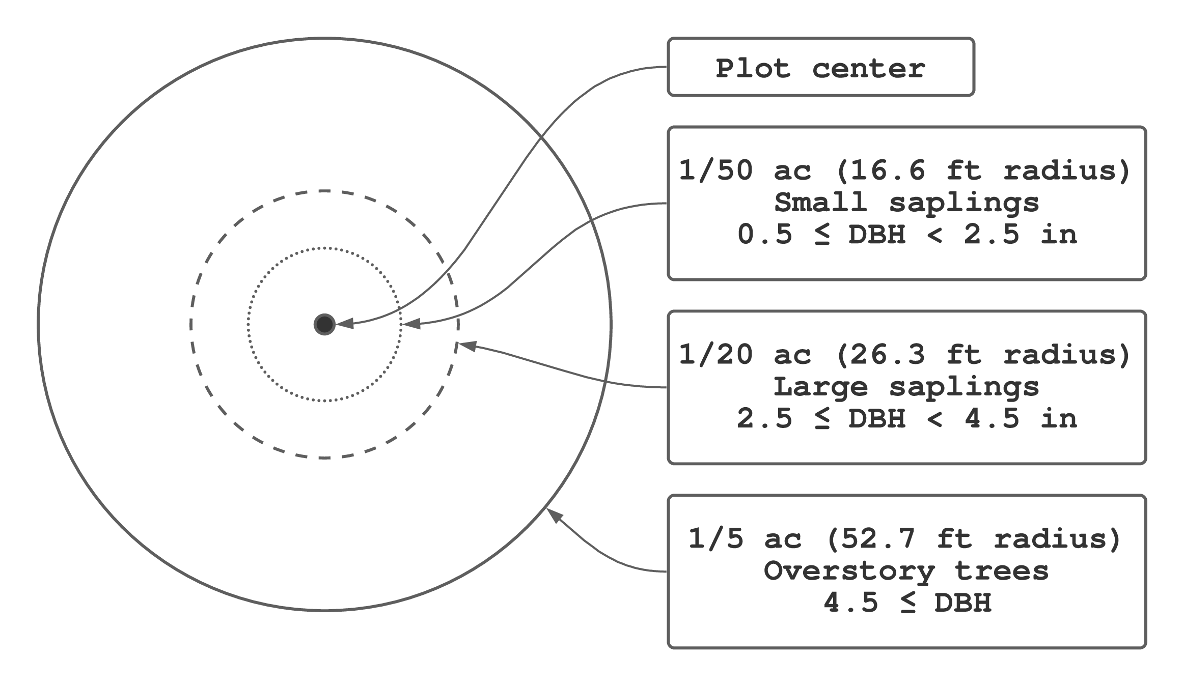
FIGURE 13.12: Penobscot Experimental Forest permanent sample plot (PSP) nested design and tree DBH measurement protocol.
Each plot depicted in Figure 2.5 was measured using the design shown in Figure 13.12.151 As noted in Section 13.3, and illustrated using the toy inventory dataset in Section 13.6, a nested plot design that uses smaller plot size to sample smaller diameter trees reduces the time needed to conduct an inventory.
The pef_trees subset created in Exercises 13.14 and 13.15 is used in Exercises 13.16 through 13.18. For several exercises, we provide the dplyr workflow output and it’s your job to write code to reproduce the output. As always, use the pipe operator when possible.
Exercise 13.14 Consider the code below used to subset pef_trees to form pef_current_trees, which includes only the most current measurement in each plot, then answer the following questions. Hint, review the MU, plot, and inv column definitions.
- Why are
MUandplotingroup_by()?
- How does the grouped
filter(inv == max(inv))result in each MU’s most current inventory?
- How is the tibble output from
filter()grouped (i.e., before it’s piped toungroup())?
- What is the effect of
ungroup()at the end of the piped workflow?
- Why might it be a good idea to remove the grouping structure on
pef_current_trees(i.e., why did we feel the need to addungroup()to the workflow)?
Exercise 13.15 Subset pef_trees_current, created in Exercise 13.14, to include only trees in the MID study and name your resulting tibble mid_trees. Hint, following the column definitions, you’ll use study == "MID" in your filter() call. Your mid_trees should match the output below.
#> # A tibble: 2,496 × 10
#>    MU     plot   inv  year month PEF_species_code
#>    <chr> <dbl> <dbl> <dbl> <dbl>            <dbl>
#>  1 90       11    25  2011     5                4
#>  2 90       11    25  2011     5                4
#>  3 90       11    25  2011     5                4
#>  4 90       11    25  2011     5                6
#>  5 90       11    25  2011     5                6
#>  6 90       11    25  2011     5                4
#>  7 90       11    25  2011     5                4
#>  8 90       11    25  2011     5                6
#>  9 90       11    25  2011     5                6
#> 10 90       11    25  2011     5                6
#> # ℹ 2,486 more rows
#> # ℹ 4 more variables: DBH_in <dbl>, AGB_lbs <dbl>,
#> #   exp_ac <dbl>, study <chr>
To provide some context for subsequent exercises, we used the tree measurements held in mid_trees to create Figure 13.13. The subsequent exercises explore these data and generate plot- and MU-level biomass estimates.

FIGURE 13.13: Penobscot Experimental Forest (PEF) management units (MUs) that are part of the Management Intensity Demonstration (MID) study are delineated in orange and labeled. Other PEF MUs are shaded gray. MID MUs are positioned near the middle of the PEF extent shown in Figure 2.5. MID permanent sample plot locations are colored by the most recent inventory’s total biomass per-acre estimate for overstory trees.
Exercise 13.16 Using mid_trees, write code to reproduce the answer to each question below.
How many trees were measured across all plots? Hint, we used
nrow().#> [1] 2496What are the distinct MU values? Hint, consider
distinct().#> # A tibble: 6 × 1 #> MU #> <chr> #> 1 90 #> 2 91 #> 3 92 #> 4 93A #> 5 93B #> 6 93CWhat year was each MU inventoried? Hint, our code uses
group_by(),summarize(), andfirst()to create theinventory_yearoutput column.#> # A tibble: 6 × 2 #> MU inventory_year #> <chr> <dbl> #> 1 90 2011 #> 2 91 2011 #> 3 92 2011 #> 4 93A 2010 #> 5 93B 2010 #> 6 93C 2010How many plots in each MU? Hint, our code uses
group_by(),summarize(), andn_distinct()to create then_plotsoutput column.#> # A tibble: 6 × 2 #> MU n_plots #> <chr> <int> #> 1 90 6 #> 2 91 6 #> 3 92 6 #> 4 93A 2 #> 5 93B 2 #> 6 93C 2How many unique plots were measured across all MUs? Hint, our code uses
summarize()andn_distinct()to create then_plotoutput column.#> # A tibble: 1 × 1 #> n_plots #> <int> #> 1 24Which three plots have the most trees measured? Hint, our code uses
group_by(),summarize()with the argument.groups = "drop", andslice_max()with the argumentn = 3.#> # A tibble: 3 × 3 #> MU plot n_trees #> <chr> <dbl> <int> #> 1 93C 12 214 #> 2 93B 12 199 #> 3 92 11 160
Exercise 13.17 As noted in the column definitions, exp_ac is the tree expansion factor (i.e., tree factor) as defined in Section 13.3.1. Use mid_trees to answer the following questions about the expansion factor.
Print the distinct values of
exp_ac. Are they consistent with the plot areas given in Figure 13.12?What is the interpretation of the
exp_acvalues? What determines a tree’s expansion factor?For each
exp_acvalue, what are the minimum and maximum DBH values? Write the code to reproduce our output below. Hint, we usedgroup_by()andsummarize()to create themin_DBH_inandmax_DBH_inoutput columns. Are the DBH ranges for each expansion factor consistent with the sampling protocol given in Figure 13.12?#> # A tibble: 3 × 3 #> exp_ac min_DBH_in max_DBH_in #> <dbl> <dbl> <dbl> #> 1 5 4.5 31.1 #> 2 20 2.5 4.4 #> 3 50 0.5 2.4
Exercise 13.18 This next series of questions results in plot-level summaries then MU-level estimates for per-acre number of trees, basal area, and aboveground biomass (AGB). We’ll limit our estimates to overstory trees in mid_trees (i.e., trees measured on the 1/5-th ac plot depicted in Figure 13.12).
After question (a) below, that filters only overstory trees, this exercise follows the estimation steps laid out in Section 13.6; however, it breaks Step 1 into two parts. The first part, question (b), expands each tree’s variable value to the per-unit-area basis. The second part, question (c), sums each tree’s values computed in question (b) to arrive at the plot-level summaries. In practice, we can combine these two parts, as we did in Section 13.6.
Filter
mid_treesto include only those trees measured on the 1/5-th ac plots and call the resulting tibblemid_overstory_trees. Yourmid_overstory_treesshould match the output below. Usemid_overstory_treesfor questions b-e.#> Rows: 1,366 #> Columns: 10 #> $ MU <chr> "90", "90", "90", "90", "90"… #> $ plot <dbl> 11, 11, 11, 11, 11, 11, 11, … #> $ inv <dbl> 25, 25, 25, 25, 25, 25, 25, … #> $ year <dbl> 2011, 2011, 2011, 2011, 2011… #> $ month <dbl> 5, 5, 5, 5, 5, 5, 5, 5, 5, 5… #> $ PEF_species_code <dbl> 6, 6, 4, 6, 6, 4, 6, 4, 4, 4… #> $ DBH_in <dbl> 13.9, 9.3, 16.1, 7.1, 17.6, … #> $ AGB_lbs <dbl> 1207.12, 445.32, 1585.07, 22… #> $ exp_ac <dbl> 5, 5, 5, 5, 5, 5, 5, 5, 5, 5… #> $ study <chr> "MID", "MID", "MID", "MID", …Add the following new columns to
mid_overstory_trees: 1)trees_per_acis the number of trees per acre each tree represents; 2)BA_sqft_per_acis the basal area (ft\(^2\)/ac) each tree represents; 3)AGB_tons_per_acis the aboveground biomass (tons/ac) each tree represents. Note you’ll need to scaleAGB_lbsby 1/2000 to convert from pounds to tons. Hint, our code usesmutate().# Take a glimpse of only a few columns so they fit on the page. mid_overstory_trees %>% select(MU, plot, trees_per_ac, BA_sqft_per_ac, AGB_tons_per_ac) %>% glimpse()#> Rows: 1,366 #> Columns: 5 #> $ MU <chr> "90", "90", "90", "90", "90",… #> $ plot <dbl> 11, 11, 11, 11, 11, 11, 11, 1… #> $ trees_per_ac <dbl> 5, 5, 5, 5, 5, 5, 5, 5, 5, 5,… #> $ BA_sqft_per_ac <dbl> 5.2688, 2.3586, 7.0687, 1.374… #> $ AGB_tons_per_ac <dbl> 3.01781, 1.11329, 3.96267, 0.…Compute the plot-level summaries by summing each plot’s values for
trees_per_ac,BA_sqft_per_ac, andAGB_tons_per_ac. Call the resulting tibbleplot_summary. We append_ito the resulting variables to indicate that they correspond to the \(i\)-th plot. Hint, our code usesgroup_by()andsummarize().152#> Rows: 24 #> Columns: 5 #> Groups: MU [6] #> $ MU <chr> "90", "90", "90", "90", "90", "90", "… #> $ plot <dbl> 11, 12, 21, 31, 51, 52, 11, 21, 31, 4… #> $ trees_i <dbl> 150, 155, 160, 250, 225, 175, 235, 28… #> $ BA_i <dbl> 109.483, 114.765, 98.615, 78.641, 160… #> $ AGB_i <dbl> 58.337, 62.491, 53.709, 37.326, 89.59…Use the plot-level summaries for MUs 90, 91, and 92 in
plot_summaryfrom question (c) to estimate MU-level mean, standard error of the mean, and 95% confidence intervals for number of trees, basal area, and AGB per acre. This is Step 2 in the estimation process described in Section 13.6.In your calculations, use the standard error given in (12.21). Call your resulting tibble
MU_estimates. Hint, our code uses onlyfilter()andsummarize().#> Rows: 3 #> Columns: 15 #> $ MU <chr> "90", "91", "92" #> $ n <int> 6, 6, 6 #> $ t <dbl> 2.5706, 2.5706, 2.5706 #> $ trees_bar <dbl> 185.83, 263.33, 247.50 #> $ s_trees_bar <dbl> 17.001, 36.370, 22.721 #> $ ci_lower_trees <dbl> 142.13, 169.84, 189.09 #> $ ci_upper_trees <dbl> 229.54, 356.83, 305.91 #> $ y_bar_BA <dbl> 117.412, 138.905, 78.939 #> $ s_BA_bar <dbl> 12.1158, 22.9370, 7.3206 #> $ ci_lower_BA <dbl> 86.267, 79.943, 60.121 #> $ ci_upper_BA <dbl> 148.556, 197.866, 97.757 #> $ AGB_bar <dbl> 63.425, 73.671, 36.802 #> $ s_AGB_bar <dbl> 7.5995, 13.0970, 3.7803 #> $ ci_lower_AGB <dbl> 43.889, 40.004, 27.084 #> $ ci_upper_AGB <dbl> 82.960, 107.338, 46.519What was the sample size used to compute your MU-level estimates in question (d)? Do you think these sample sizes are large enough to provide robust estimates?
Use the MU-level estimates in
MU_estimatesfrom question (d) to compute MU-level total with associated 95% confidence intervals for AGB.153 MU 90, 91, and 92 have an area of 9.92, 9.76, and 9.92 acres, respectively. Break your workflow into three steps. First, make a tibble calledmu_acreswith columnsMUandA_ac, whereA_acholds the acres for each MU. Second, joinmu_acrestoMU_estimates.154 Third, usemutate()ortransmute()onMU_estimatesto create a tibble that holds AGB estimated total and associated confidence intervals. The output from these three steps is given below.Step 1: Create the
mu_acrestibble.#> # A tibble: 3 × 2 #> MU A_ac #> <chr> <dbl> #> 1 90 9.92 #> 2 91 9.76 #> 3 92 9.92Step 2: Join
mu_acrestoMU_estimates.Step 3: Use
MU_estimatesandtransmute()to estimate AGB total with associated confidence interval. Name the resulting tibbleMU_tot_estimates. Hint, scale the per-unit-area estimates by their respective MU acres.#> Rows: 3 #> Columns: 4 #> $ MU <chr> "90", "91", "92" #> $ AGB_hat <dbl> 629.17, 719.03, 365.07 #> $ ci_lower_AGB <dbl> 435.38, 390.44, 268.68 #> $ ci_upper_AGB <dbl> 822.96, 1047.62, 461.47
References
We use forest generically to represent a bounded land area holding the population of interest.↩︎
The plot defining each tree’s inclusion zone is created by replicating the plot intended for the sampling location, rotating it 180\(^\circ\), and positioning it at the tree’s location; see Chapter 7 in Gregoire and Valentine (2008) for further explanation and examples. The inclusion zone rotation is not apparent in Figure 13.1(b) because the circular plot is symmetric about the sampling location.↩︎
Often referred to as a milacre plot.↩︎
Calculation of basal area from DBH and derivation of the constant \(c\) under English and metric systems are in Section 6.3.1.↩︎
Here and throughout the remainder of the book, we intentionally retain more digits than would normally be reported. This makes intermediate calculations easier to follow and helps verify results using independent calculations or software. In practice, final estimates would be rounded to a sensible number of significant digits.↩︎
By standard order-of-operations rules (reviewed in Section 11.2), each tree measurement \(y_{ij}\) is first multiplied by its tree factor \(\text{TF}_{ij}\), and the resulting products are then summed over trees on plot \(i\). When in doubt, it’s always worth pausing to check the implied order.↩︎
You might ask, “If all trees are measured on the same plot area, why complicate life with this \(j\) subscript for tree-specific TF?” There are a several good reasons. First, as noted earlier, it’s common to have more than one plot size in a given inventory, e.g., a plot for overstory trees and a nested subplot for regeneration, so the dataset includes trees with different TFs. Second, as developed later in Section 13.4, under point sampling a tree’s inclusion zone depends on its size (e.g., its basal area), so TF differs by tree. Third, using a tree-specific TF supports an efficient workflow developed in Section 13.6 that works for both plot and point sampling.↩︎
Paul Schmid published his original mirage method development in German. Later, an English publication by Beers (1977) highlighted Schmid’s method and proposed an extension for settings where the mirage method could not be implemented.↩︎
R’s trigonometric functions assume angles are in radians, not degrees. To reproduce this example in R using
cos(), first convert the angle from degrees to radians with thed2r()function:d2r <- function(d) { d * pi / 180 }. So for the \(C_1\) example:26.33/cos(d2r(30)). Other useful angle conversion functions are listed in Exercise 13.12.↩︎Like the Harvard Forest census dataset, it’s useful to learn about different estimators and associated computations using a census because it allows you to check your resulting estimates against the truth. Clearly, this is never a luxury we have when sampling a real population.↩︎
Because much of the field activity occurs at the overstory plot center (e.g., holding the tape while checking in/out trees and setting permanent plot markers), regeneration subplots are typically offset from this high-traffic area to avoid trampling seedlings before they can be measured.↩︎
Get used to these steps—they’re a recurring theme in forest inventory data analysis.↩︎
Calculation of basal area from DBH and derivation of the constant \(c\) under English and metric systems are in Section 6.3.1.↩︎
Later in the book, we introduce variants such as Big BAF sampling (Section 17.5), where DBH is measured on only a subset of the counted trees to support estimation of additional parameters, while retaining the basic point-sampling framework.↩︎
Bitterlich’s angle count method is also known as Bitterlich sampling, prism sampling, plot-less sampling, variable radius plot sampling, variable plot sampling, and plotless cruising.↩︎
This statement holds when a tree’s inclusion zone lies fully within the boundary. When any portion of the zone falls outside the boundary, the tree has a reduced probability of selection, leading to boundary slopover bias and the need for corrective methods (Section 13.3.3).↩︎
Interestingly, they found that even though errors were made by professional cruisers in calling borderline trees as “in” or “out,” the errors tended to cancel over the entire cruise. Those errors that didn’t cancel out (i.e., bias) were typically due to inaccurate slope corrections and line of sight issues. Inexperienced cruisers tended to make more non-canceling errors. The authors strongly recommend measuring all potential borderline trees.↩︎
While any area unit can be used, we focus on acres and hectares because they’re most commonly used in forestry applications.↩︎
Equation (13.19) is identical to (13.2); we repeat it here for convenience.↩︎
Remember, you choose the angle \(\theta\), or perhaps it’s chosen for you and specified in the survey protocol.↩︎
Notice we dropped the \(j\) subscript on BAF. This is because a single BAF is typically used for a given population—more on this topic in Section 13.4.3.↩︎
There are a few exceptions where point-level summaries can be obtained without tree factors—see Section 13.4.6.↩︎
In English units, the analogous simplification is \(R = \frac{\sqrt{10890}}{12}\cdot\frac{\text{DBH}}{\sqrt{\text{BAF}}} \approx \frac{8.696\cdot\text{DBH}}{\sqrt{\text{BAF}}}\), which is far less tidy than the metric identity. This is why English-unit practice typically relies on tabulated HDMs, or computes \(k\) via (13.26) and then plugs it into (13.27) to get \(R\).↩︎
If you want to reproduce the constant \(k\) in Tables 13.7 and 13.6 in R using (13.13), convert the angle \(\theta\) from degrees to radians with the
d2r()function:d2r <- function(d) { d * pi / 180 }. Recall from Section 13.3.4 that R’s trigonometric functions assume angles are in radians, not degrees.↩︎Calculations for the constant \(c\) are given in Section 6.3.1.↩︎
International 1/4-inch log rule estimates board feet from a log, accounting for stem taper, wood removed from the outside of the log to square it off, and saw kerf (or the loss of wood as sawdust), see, e.g., USDA (2006).↩︎
Check your understanding by computing other VBARs in Table 13.13 using values in Table 13.12.↩︎
The line’s slope is found using the least-squares regression method with a zero intercept constraint, implemented using the
lm()function; see Section 17.1 for more details.↩︎This is especially true if trees are measured on different sized plots or under point sampling where the tree factor depends on tree-specific characteristics like DBH.↩︎
Notice again that
plot_summaryis already grouped bystand_id, so the subsequent call tosummarize()produces stand-level summaries, as desired.↩︎With only two stands, it’s simple enough to use
case_when()withinmutate()to add stand-specific information like area. For larger datasets, a more flexible and scalable approach is to use a mutating join (Section 8.14.1) to merge stand attributes with plot- or stand-level summaries. For example, see howleft_join()is used for this purpose in Section 16.7.↩︎Because the same BAF was used for both stands, we could have simply referenced the
BAFvariable defined outsideo_stands. However, it’s common to have stand-specific BAF values, in which case you’d want to include aBAFcolumn in your dataset. You could usecase_when()to assign stand-specific values.↩︎After running the code below, you can confirm that Plot 2 is still present as a factor level by calling
levels(o_stand$plot_id).↩︎This design, detailed in Waskiewicz et al. (2015), was only consistently applied to recent PEF data. If you dig into the
pef_treesdata, you’ll find that prior to 2000 many tree measurements don’t follow the DBH cutoffs given in Figure 13.12.↩︎As an aside, plot color in Figure 13.13 corresponds to the
AGB_ivalue in your resultingplot_summarytibble.↩︎We could also compute the totals for number of trees and basal area; however, in practice we typically talk about these variables on a per-unit-area basis.↩︎
We used
case_when()to accomplish these first two steps in Section 13.6.1. We’re using the join approach here for demonstration—it’s a better approach in practice when you’re dealing with many units that need values assigned.↩︎