Chapter 11 Preliminary definitions and concepts
Translating mathematical expressions found in publications and reference material into code is a fundamental data analyst skill. This chapter defines terminology and mathematical notation used throughout the remainder of the book to introduce statistical concepts and how they can be translated into efficient analysis workflows.
11.1 Estimating population parameters
A central aim of data analysis, as covered in this book, is to infer (meaning to deduce or learn about) population characteristics of interest from a sample taken from the population. The population is an aggregate of units that belong to some defined group. The units are individuals or objects that collectively comprise the population. In some cases we’re able to observe (meaning measure) all units in the population. Observing all population units is a census and means we can describe the population characteristic of interest in its entirety and without error (assuming no measurement error). Recall, the Harvard Forest dataset described in Section 2.2.5 is a census of the population, with units defined as all woody vegetation with a DBH of 1 cm and larger. In most practical cases, however, it’s too time-consuming or expensive to observe all units in the population. In such cases, we settle for observing a sample, which means a subset of population units. If selected appropriately, this sample might ultimately provide a useful estimate of the population characteristic of interest.
We use the word parameter to mean a summary measure of a population characteristic. For example, a parameter could be an average, total, or proportion. Similarly, we use the word statistic to mean a summary measure of a sample characteristic, and like a parameter, a statistic could be an average, total, or proportion. Statistics are used to infer something about the population parameter of interest.
A characteristic that might vary from unit to unit is called a variable. Our observations, or measurements, of a variable in a sample of population units inform statistics, which serve as estimates of the population parameter of interest. The typical data analysis progression takes the following steps.
- Define the population, population units, and population parameters of interest, then
- Measure one or more variables on a sample of population units, and compute one or more statistics that serve as estimates of the population parameters. Typically, these statistics provide our best estimate of the parameter and quantify how certain we are in the estimate.
Here’s an example to illustrate this new vocabulary. Say you want to know the total merchantable timber volume on a 50-acre property, where you define “merchantable timber volume” as volume from live trees 10.0 inches DBH or larger with at least one 16-foot sawlog. The population comprises all trees that meet your definition of merchantable timber volume on the 50-acre property. The population parameter of interest is total merchantable timber volume. The population units are the individual trees that meet your merchantable definition. The variable measured on each unit (i.e., tree) is its volume.93
Alternatively, and more typically in practice, we might define the population units as some fixed-area field plot. For example, we might divide the 50-acre property into 250 1/5-th acre non-overlapping plots. In this case, the variable is the cumulative volume of all trees that meet the population definition for merchantable timber on each 1/5-th acre plot. Regardless of whether our population unit is an individual tree or a group of trees on a plot, we likely won’t be able to take a census of the property due to time or effort constraints, but rather we’ll select a sample of population units for which we’ll measure volume. Then, given the sample measurements, we compute a statistic that serves as our estimate for total merchantable timber volume on the property.
11.1.1 Types of variables
It’s useful to connect the R data types introduced in Section 5.2.1 with those of variables we encounter in subsequent chapters. Following Figure 11.1, a variable is initially classified as either quantitative or qualitative.
A quantitative variable has values that give a notion of magnitude; that is, the values are a numerical measure. This numerical measure is either continuous or discrete. A quantitative continuous variable can take an infinite (not countable) number of possible values, i.e., an infinitely fine increment from one value to the next. Said differently, a continuous variable can have an arbitrary number of decimal places for a given value. Examples include height, weight, and volume. In comparison, a quantitative discrete variable can take a finite (countable) number of possible values when moving from one value to the next. The values are often (but not always) integers. Examples include age in whole years, number of trees, and number of fire events.
A qualitative variable (also referred to as a categorical variable) has values that represent different categories. Qualitative variables are either nominal or ordinal. A qualitative nominal variable takes values for which no ordering is possible or implied in the categories. For example, the variable species is nominal because there’s no inherent or natural order in species names. Similarly, forest ownership type coded as federal, state, private, or tribal is nominal because there’s no apparent ordering. In contrast, the categories of a qualitative ordinal variable have some natural ordering. For example, the variable tree canopy position can take the values suppressed, intermediate, co-dominant, or dominant, where these categories themselves imply an ordering. Further examples include disturbance severity code with categories low, medium, and high, or forest or ecosystem succession stages. Again, in these examples, there is a natural order to the categories.
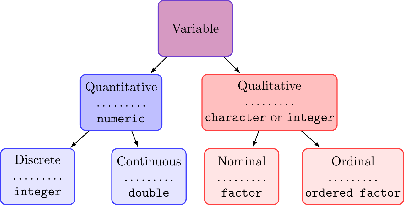
FIGURE 11.1: Variable types with corresponding R data types added below the dotted line.
11.2 Tools of the trade: Review of notation
Frank Freese was a prolific forest biometrician who worked for the USFS Southern Experiment Station in Asheville, North Carolina, and the Forest Products Lab in Madison, Wisconsin. He wrote several primers on applied statistics for practicing foresters. Despite being somewhat dated, Frank’s works are clearly written, fun to read, and offer lots of worked examples that make them enduring resources for those interested in an efficient and accessible introduction to classical statistics and sampling methods. In one of his works entitled Elementary Forest Sampling (Freese 1962), he includes a section called “Tools of the Trade: Subscripts, Summations, and Brackets” that provides a refresher (or perhaps a first look) at more frequently used mathematical expressions in applied statistics and sampling. Following Frank’s lead, we offer a similar section that covers common mathematical notation and its translation to R code.
Throughout the remainder of this book, Greek letters, e.g., \(\mu\), \(\sigma\), \(\alpha\), \(\beta\), \(\eta\), represent population parameters.94 Roman letters, e.g., \(x\), \(y\), \(z\), represent variables. For example, we might say \(x = 5\), which is a scalar (i.e., single value), or \(y = (1,4,5)\), which is a vector of three values. A vector is a collection of one or more values organized such that the values can be referenced using an index—analogous to the R vector data object introduced in Section 5.2. A sample statistic, which is any quantity computed from values in a sample and used to estimate population parameters, will be represented using a Roman letter, sometimes decorated with a bar, hat, or some other symbol. For example, \(\bar{y}\) is read as y bar and \(\hat{R}\) as R hat.
11.2.1 Mathematical operators, subscripts, and nested data
You already know many mathematical operators: addition +, subtraction -, multiplication *, division \, exponentiation ^, and assignment =. Like the comparison and logical operators introduced in Section 5.7, mathematical operators are applied to operands. For example, in the expression 1 + 2, there are two operands: the left operand is 1 and the right operand is 2. An operator is binary if it has two operands and unary if it has a single operand.
Although you might not have thought about it this way, the minus sign - can be unary (negation) or binary (subtraction). The unary form reverses the sign of the operand on its right; the binary form subtracts the right operand from the left.
Subscripts appear as one or more letters to the lower right side of a variable. For example, \(x_{i}\) is a variable \(x\) with subscript \(i\). The subscript letter is a placeholder for an integer value used to index elements in a vector. Say \(x=(4,1,5,2,8)\); that is, the variable \(x\) is a vector of length 5 with values 4, 1, 5, 2, and 8. If \(i = 1\), then \(x_i\) equals 4—the first element in the vector. Similarly, when \(i = 2\), \(x_i\) equals 1; when \(i = 3\), \(x_i\) equals 5; and so on.
You’ll see in later chapters that summing the elements of a vector is a recurring theme when computing sample statistics and other quantities of interest. Following from the previous example, the sum of the vector \(x\) could be written as
\[\begin{equation*}
(x_1 + x_2 + x_3 + x_4 + x_5).
\end{equation*}\]
A more compact way to write this summation is
\[\begin{equation*}
(x_1 + x_2 + \ldots + x_5),
\end{equation*}\]
where the \(\ldots\), which is an ellipsis, means to continue the same pattern for \(x_3\) and \(x_4\). An even more compact way to express this summation is
\[\begin{equation*}
\sum^5_{i=1}x_i,
\end{equation*}\]
where \(\sum\) is a symbol that means add a + between the values of \(x_i\) each time \(i\) changes. The \(i=1\) below the summation symbol says subscript \(i\) starts at value 1 and increases by 1 until it equals the number above the summation symbol, which in this case is 5. In some books, you’ll see the number on top of the summation symbol omitted, which should be taken to mean increment the subscript to the number of elements in the vector being summed.
Very often we use more than one subscript to reference values of a variable. For example, from Section 2.2.1, recall the FEF dataset comprises 88 trees sampled on 17 plots across two watersheds. More specifically, 44 trees were measured across 8 plots in watershed 1, and 44 trees were measured across 9 plots in watershed 2. We’ll see later that it’s helpful to use a separate subscript to index each level in these kinds of nested datasets.
For now, let’s just focus on the data in one of the two watersheds. Let \(x\) represent stem biomass and use subscript \(i\) for plot and \(j\) for tree. Using this notation, we can uniquely identify any tree biomass using the subscript \(x_{i,j}\). Translating this notation into words, we might say \(x_{i,j}\) is the biomass of the \(j\)-th tree in the \(i\)-th plot. Now, using these subscripts, say we want the total biomass of all trees across all plots, which can be written \[\begin{equation*} \sum^{m}_{i=1}\sum^{n_i}_{j=1}x_{i,j}, \tag{11.1} \end{equation*}\] where \(m\) is the number of plots and \(n_i\) is the number of trees in plot \(i\). Notice the subscript on \(n\) is necessary because there might be a different number of trees in each plot, and the \(i\) says that \(n_i\) is plot-specific. The expanded equivalent of this summation is \[\begin{align*} x_{1,1}&+x_{1,2}+\ldots +x_{1,n_1}\nonumber\\ +&x_{2,1}+x_{2,2}+\ldots +x_{2,n_2}\nonumber\\ &\quad\quad\quad\quad\quad\vdots\nonumber\\ +&x_{i,1}+x_{i,2}+\ldots +x_{i,n_i}\nonumber\\ &\quad\quad\quad\quad\quad\vdots\nonumber\\ +&x_{m,1}+x_{m,2}+\ldots +x_{m,n_m}, \tag{11.2} \end{align*}\] where the \(\vdots\) indicates that each omitted row in the expression looks the same as the first two, except that they increment the \(i\) index until it reaches \(m\).
| Plot (\(i\)) | Tree (\(j\)) | \(x\) | \(y\) |
|---|---|---|---|
| 1 | 1 | 1.2 | 3 |
| 1 | 2 | 2.4 | 4 |
| 2 | 1 | 0.4 | 2 |
| 2 | 2 | 6.3 | 6 |
| 2 | 3 | 2.2 | 5 |
Consider the example data given in Table 11.1. Using the same notation as the FEF biomass summation example above, these example data comprise \(m=2\) plots (indexed using \(i\)), with multiple trees measured in each plot (indexed using \(j\)). For plot \(i=1\), there are \(n_i=2\) trees measured, and for plot \(i=2\), there are \(n_i=3\) trees measured. The columns \(x\) and \(y\) represent two variables measured on each tree.
Using the indexing described above, the sum of the \(x\) values in Table 11.1 can be written as \[\begin{align*} \sum^{m}_{i=1}\sum^{n_i}_{j=1}x_{i,j}&=x_{1,1}+x_{1,2}+x_{2,1}+x_{2,2}+x_{2,3}\\ &=1.2+2.4+0.4+6.3+2.2\\ &=12.5. \end{align*}\]
This subscript notation extends in a straightforward way to accommodate any number of different data levels combined with any mathematical operator (we focus on the summation operator here because it’s used most frequently in the methods considered in this book). As an example of extending this notation, consider the watershed level of the FEF data and index watershed using subscript \(h\), with \(H\) representing the number of watersheds. Tree biomass measurements \(x\) can now be indexed as the \(j\)-th tree, within the \(i\)-th plot, within the \(h\)-th watershed. The total biomass is now expressed as \[\begin{equation} \sum^{H}_{h=1}\sum^{m_h}_{i=1}\sum^{n_i}_{j=1}x_{h,i,j}. \tag{11.3} \end{equation}\] Note that in the summation above we added the \(h\) subscript to \(m\) to acknowledge that there might be a different number of plots within each watershed.
A common characteristic of datasets we encounter is that tree measurements (i.e., observations) are nested in one or more levels. The FEF data are a perfect example: observations are nested in plots, plots are nested in watersheds, and the watersheds are nested in the entire FEF. The Elk County inventory data in Section 2.2.2 have tree observations nested in plots, which are nested in the forested property. The PEF data in Section 2.2.4 have tree observations nested in year, nested in inventory plot, nested in management unit, and the management units are nested in the entire PEF. The FACE data in Section 2.2.3 have a complex nesting structure, with aspen tree diameter observations nested in clone, nested in year, nested in experimental replicate, and nested in treatment. As illustrated in (11.3), subscripts provide useful notation to describe how observations are nested at different levels and the order in which different mathematical operators apply to the observations. This nesting becomes especially important in the programming and analysis chapters, where we apply different estimators and seek data summaries at various data levels.
As demonstrated in subsequent chapters, the dplyr group_by() and summarize() workflows, along with other tidyverse functions, are perfectly suited to efficiently analyzing the kind of nested data we encounter in practice.
11.2.2 Order of operations
Perhaps at one time you learned the acronym PEMDAS for Parenthesis, Exponents, Multiplication, Division, Addition, and Subtraction, along with its handy mnemonic Please Excuse My Dear Aunt Sally. Given two or more operations in a single expression, the order of the letters in PEMDAS tells us what to calculate first, second, third, and so on, until the calculation is complete. Confusing the order of operations is a common coding error when implementing the estimators considered in subsequent chapters—it’s time well invested reviewing and practicing these foundational rules.
Consider the summation of \(n\) values of a variable \(x\) squared, expressed as \[\begin{equation} \sum^n_{i=1}x_i^2. \tag{11.4} \end{equation}\] The two operations in (11.4) are raising each \(x_i\) to the exponent of 2 (i.e., squaring), and summing the \(n\) resulting values of \(x_i^2\). Here, our handy acronym PEMDAS reminds us to apply exponents before summation, so we first square each \(x_i\) and then sum the resulting \(n\) values.
Now let’s add parentheses around the summation in (11.4) and see how the order of operations changes \[\begin{equation} \left(\sum^n_{i=1}x_i\right)^2. \tag{11.5} \end{equation}\] Looking at (11.5) and applying PEMDAS, the order of operations is to first sum the \(n\) \(x\) values because they are inside parentheses, then square the scalar result. A scalar is a mathematical term meaning a single real number, which is what you’re left with after the summation in (11.5).
Following the data structure in Table 11.1, consider the expression \[\begin{equation} \sum^m_{i=1}\left(\sum^{n_i}_{j=1}x_{i,j}\right)^2, \tag{11.6} \end{equation}\] where, recall, \(i\) indexes the \(m\) plots and \(j\) indexes the \(n_i\) trees on each plot. There are a few steps to evaluate (11.6). First, for each value of \(i\), sum over the \(n_i\) values of \(x_{i,j}\), then square the resulting scalar. Second, sum the \(m\) resulting scalars. Here’s the expanded form: \[\begin{align} \sum^m_{i=1}\left(\sum^{n_i}_{j=1}x_{i,j}\right)^2= &\left(x_{1,1}+x_{1,2}+\ldots+x_{1,n_1}\right)^2\nonumber\\ &+\left(x_{2,1}+x_{2,2}+\ldots+x_{2,n_2}\right)^2\nonumber\\ &\quad\quad\quad\quad\quad\vdots\nonumber\\ &+\left(x_{m,1}+x_{m,2}+\ldots+x_{m,n_m}\right)^2. \tag{11.7} \end{align}\] Using data in Table 11.1, (11.7) equals 92.17.
From here forward, we’ll drop the comma between subscript elements (e.g., \(x_{i,j}\)) to reduce visual clutter. The comma is handy when first introducing subscripts because it clearly separates multiple indices and helps explain subsetting. However, as equations grow longer the comma adds nothing to meaning and only clutters the notation, so we’ll omit it to keep expressions cleaner and easier to read.
You might also encounter two or more variables with subscripts in the same expression. For example, \[\begin{equation} \sum^n_{i=1}x_iy_i = x_1y_1 + x_2y_2 + \ldots + x_ny_n, \tag{11.8} \end{equation}\] where, following PEMDAS, multiplication of \(x_i\) and \(y_i\) comes before summation.
Here’s another expression with two variables \[\begin{equation} \left(\sum^n_{i=1}x_i\right)\left(\sum^n_{i=1}y_i\right) = (x_1 + x_2 + \ldots + x_n)(y_1 + y_2 + \ldots + y_n), \tag{11.9} \end{equation}\] where, because of the parentheses, we first sum the \(n\) values of \(x\) and \(y\), then multiply the two resulting scalars.
11.2.3 Tools of the trade using R
As noted at the beginning of Section 11.2, a vector is a collection of one or more values organized so they can be referenced using an index. Since we’re talking about mathematical operations here, it’s implied the vector elements are numeric. We saw in Section 3.1.1 that a vector is created using the c() function. We use this function again to make a vector x using the \(x\) values in Table 11.1.
Recall from Section 5.2, we access vector elements using their position or index in square brackets, starting with 1 for the first element and ending with length(x) (equivalent to 5) for the last element. For example, x[1] is 1.2, x[2] is 2.4, and x[5] is 2.2. Notice these indexes follow the mathematical subscript notation introduced above and are equivalent to \(x_1\), \(x_2\), and \(x_5\).
R applies unary operators to all elements in a vector. In the code below, we see how the unary negation operator changes the sign of all elements.
#> [1] -1.2 -2.4 -0.4 -6.3 -2.2Note the code above only changes the sign of the printed values, not the values in x. If you want to change the values in x, you need to assign the negated vector back to x.
#> [1] -1.2 -2.4 -0.4 -6.3 -2.2#> [1] 1.2 2.4 0.4 6.3 2.2A binary operator between two vectors of the same length takes the left and right operands from each element along the vectors (an elementwise operation). This is illustrated in the elementwise multiplication of the \(x\) and \(y\) variables from Table 11.1.
#> [1] 3.6 9.6 0.8 37.8 11.0Here’s a very important concept we initially touched upon in Sections 5.2.3 and 5.7. For elementwise operations involving two or more vectors, the vectors must be the same length. If R encounters two vectors of different lengths in a binary operation, it replicates (recycles) the smaller vector until it’s the same length as the longest vector, then performs the operation.
For example, say we scale the vector x by 5, i.e., 5 * x. Recall, R stores single values as a vector of length 1, so the 5 is replicated length(x) times before the elementwise multiplication.
Consider another example where the vector z (defined in the code below) is shorter than x. Since x is the longer vector (length 5), z is recycled until it matches the length of x, so z will be 1, 2, 1, 2, 1. Because the length of x is not a multiple of the original length of z, the recycled z is truncated and R kindly prints a warning, but still returns the result, as illustrated below.
#> Warning in x + z: longer object length is not a
#> multiple of shorter object length
#> [1] 2.2 4.4 1.4 8.3 3.2R follows the PEMDAS order of operations. Take a moment to study R’s precedence of operators manual page, accessed via ?Syntax. The manual page lists operators in precedence groups, from highest (applied first) to lowest (applied last). You’ll see that the PEMDAS ordering is reflected in the manual page’s precedence ordering, and in how these mathematical operators are positioned relative to other R operators and syntax.
The next lines of code implement (11.4) and (11.5), respectively. Notice the sum() function is equivalent to the \(\sum\) operator, and exponentiation is done relative to the parentheses.
#> [1] 51.89#> [1] 156.25We implement (11.8) and (11.9) below.
#> [1] 62.8#> [1] 250Above, and in subsequent chapters, we often illustrate ideas using single vectors that represent measurements on a variable. However, in practice, these vectors are typically columns in a data frame. So let’s extend the order of operations examples above to variables in a data frame. We begin by moving the data in Table 11.1 to a data frame using the tibble() function, introduced in Section 7.2.
plots <- tibble(plot_index = c(1, 1, 2, 2, 2),
                tree_index = c(1, 2, 1, 2, 3),
                x = c(1.2, 2.4, 0.4, 6.3, 2.2),
                y = c(3, 4, 2, 6, 5))
Now let’s repeat the last few order of operations examples above using dplyr functions covered in Chapter 8.95 The code below computes (11.4), (11.5), (11.8), and (11.9), all in one call to summarize().
plots %>%
  summarize(`sum(x^2)` = sum(x^2),
            `sum(x)^2` = sum(x)^2,
            `sum(x*y)` = sum(x * y),
            `sum(x)*sum(y)` = sum(x) * sum(y))
#> # A tibble: 1 × 4
#> `sum(x^2)` `sum(x)^2` `sum(x*y)` `sum(x)*sum(y)`
#> <dbl> <dbl> <dbl> <dbl>
#> 1 51.9 156. 62.8 250Going back to subscripts and nested data. We’ll often want to apply the same equation to subsets of data indexed by one or more qualitative variables that indicate group membership. For example, let’s use the plot_index column in the plots data frame to apply equations to trees within each plot. This is easily done by using plot_index as a grouping variable, as illustrated below.
plots %>%
  group_by(plot_index) %>%
  summarize(`sum(x^2)` = sum(x^2),
            `sum(x)^2` = sum(x)^2,
            `sum(x*y)` = sum(x * y),
            `sum(x)*sum(y)` = sum(x) * sum(y))
#> # A tibble: 2 × 5
#> plot_index `sum(x^2)` `sum(x)^2` `sum(x*y)`
#> <dbl> <dbl> <dbl> <dbl>
#> 1 1 7.2 13.0 13.2
#> 2 2 44.7 79.2 49.6
#> # ℹ 1 more variable: `sum(x)*sum(y)` <dbl>Let’s go back and look at (11.6) and its expanded form in (11.7). Recall \(i\) indexes plot and \(j\) indexes tree within plot, \(m\) is the number of plots, and \(n_i\) is the number of trees within each plot. For the data in Table 11.1, \(m = 2\); for \(i = 1\), \(n_i = 2\); and for \(i = 2\), \(n_i = 3\).
The double summation can be completed using the following, where within_plots is the squared sum of x for each plot, and across_plots is the sum of the within_plots values.
plots %>%
  group_by(plot_index) %>%
  summarize(within_plots = sum(x)^2) %>%
  summarize(across_plots = sum(within_plots))
#> # A tibble: 1 × 1
#> across_plots
#> <dbl>
#> 1 92.2As always, it can be instructive to run the code above incrementally and compare the output of each call to summarize() with the right-hand side of (11.7).
11.3 Summary
In this chapter, we covered essential data analysis vocabulary and statistical notation used throughout the remainder of the book. We began by defining concepts related to populations, samples, and variables. We described the typical data analysis progression: define the population, population units, and the population parameter of interest, then measure one or more variables on a sample of population units and use these measurements to compute a statistic that serves as an estimate of that parameter. We’ll see more concrete examples of this workflow beginning in Chapter 12.
Next, we extended our discussion to quantitative and qualitative variables. Quantitative variables are numeric and defined as discrete (finite increment between values, e.g., an integer) or continuous (infinite increment between values, e.g., a number with decimals). Qualitative variables represent different categories and can be nominal (no order) or ordinal (ordered).
We then shifted to the notation used throughout the remainder of the book. We use Greek letters (e.g., \(\mu\), \(\sigma\)) to represent population parameters and Roman letters (e.g., \(x\), \(y\)) to represent variables, and Roman letters—sometimes decorated with bars, hats, or other symbols—to represent statistics.
We reviewed mathematical operators and discussed subscripts and their role in summations and nested data. We stressed the importance of understanding how subscripts reference variable values in a nested dataset, as nested data are extremely common in both forestry and environmental sciences.
We finished by discussing the ever-important order of operations. While it might seem conceptually straightforward, we’ve spent precious hours (even days) tracking down bugs that turned out to be simple errors caused by overlooking PEMDAS.
With tools of the trade in hand, you’re ready for Chapter 12, which develops the statistical foundations you’ll use to make inferences about populations.
11.4 Exercises
With the exception of Exercise 11.10, all exercises should be completed by hand, i.e., without using R. Use the information in Table 11.1 to complete Exercises 11.1 through 11.9.
Exercise 11.1 How many tree measurements of variable \(x\) are there for Plot 1 and Plot 2?
Exercise 11.2 Evaluate the expression \(\sum^{2}_{j=1}x_{ij}\), where \(i=1\), i.e. sum the \(x\) variable values for Plot 1.
Exercise 11.3 Evaluate the expression \(\sum^2_{i=1}\sum^{n_i}_{j=1}x_{ij}\), where \(n_i\) is the total number of trees in each plot.
Exercise 11.4 Evaluate the expression \(\sum^2_{i=1}\sum^{n_i}_{j=1}x_{ij}^2\), where \(n_i\) is the total number of trees in each plot.
Exercise 11.5 Evaluate the expression \(\sum^2_{i=1}(\sum^{n_i}_{j=1}x_{ij})^2\), where \(n_i\) is the total number of trees in each plot.
Exercise 11.6 Evaluate the expression \(\sum^2_{i=1}\sum^{n_i}_{j=1}x_{ij}y_{ij}\), where \(n_i\) is the total number of trees in each plot.
Exercise 11.7 Evaluate the expression \(\sum^2_{i=1}\sum^{n_i}_{j=1}x_{ij}^2y_{ij}\), where \(n_i\) is the total number of trees in each plot.
Exercise 11.8 Is \(\sum^n_{i=1}x_i^2\) equal to \(\left(\sum^n_{i=1}x_i\right)^2\)?
Prove your answer using the \(x\) values, with \(i\) redefined to sequentially index the \(x\) values from \(i = 1, \ldots, n\) where \(n = 5\).
Exercise 11.9 Is \(\sum^n_{i=1}x_iy_i\) equal to \(\left(\sum^n_{i=1}x_i\right)\left(\sum^n_{i=1}y_i\right)\)?
Prove your answer using the \(x\) and \(y\) values, with \(i\) redefined to sequentially index the \(x\) and \(y\) values from \(i = 1, \ldots, n\) where \(n = 5\).
Exercise 11.10 Evaluate the following expression first by hand (with the aid of a calculator), then using R:
\[
\frac{\left(\exp(14) + 10\right) \times \sqrt{5}}{\ln(4) - 5 \times 10^2},
\]
where \(\exp\) is the exponential function and \(\ln\) is the natural logarithm (i.e., \(\log_e\)), which correspond to exp() and log() in R.
References
Although in practice we typically measure DBH and height, then compute volume using an allometric equation like those briefly discussed in Section 2.2.1 and illustrated in Sections 6.3.2 and 8.14.3.↩︎
These are the letters mu, sigma, alpha, beta, and eta, respectively.↩︎
In this example we’re using non-syntactic names in
summarize(), protected with backticks (see Section 4.2.2 for naming rules). Using non-syntactic names should generally be avoided, but it’s useful here to match the mathematical expression with its resulting value.↩︎